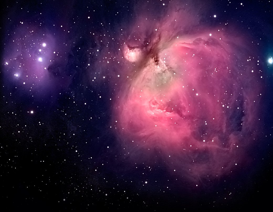
Use Case: From SED fitting to Age estimation. The case of Collinder 69 Model fit.
The determination of physical parameters of astronomical objects from observational data is
frequently linked with the use of theoretical models as templates.
The use, in the traditional way, of this methodology can easily become tedious and even
unfeasible when applied to a large amount of data. VOSA uses VO methodologies to authomatically fit
several collections of theoretical models to the observed photometry for different objects
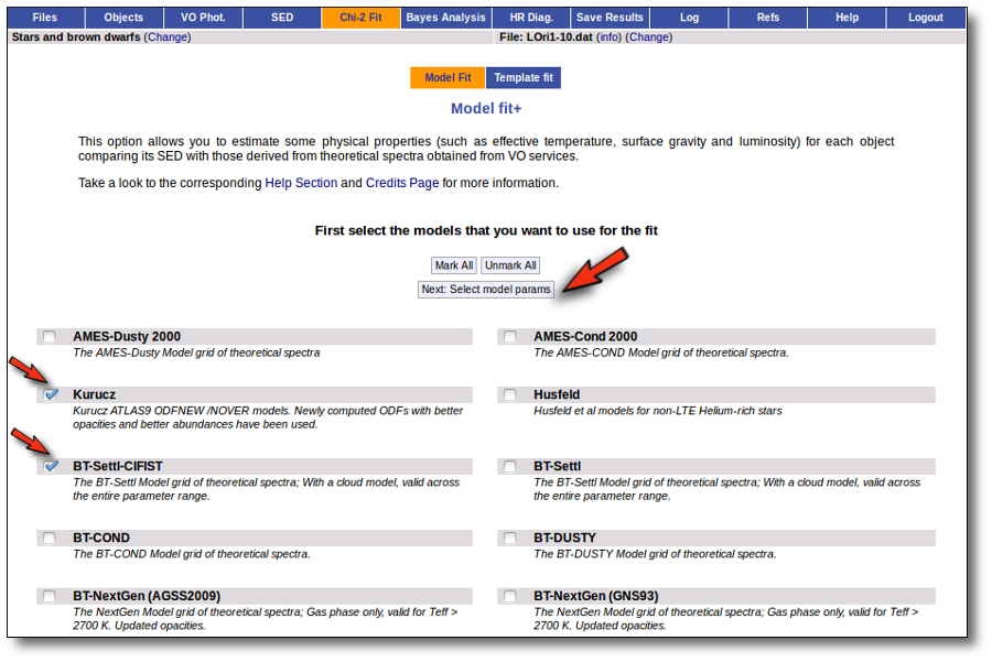
When we access the Chi-2: Model Fit tab we see a form with the available theoretical models, so that we can choose what ones we want to use in the fit. In this case we decide to try Kurucz and BT-Settl-CIFIST models. Thus, we mark them and click in the "Next: Select model params" button.
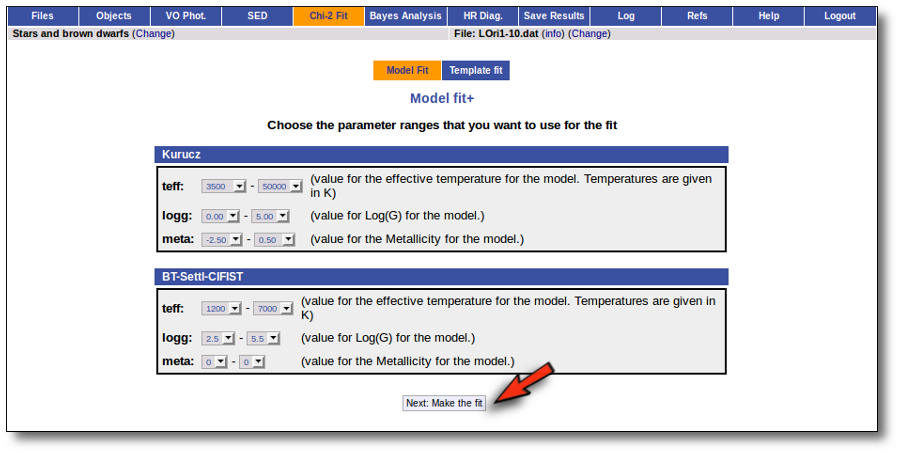
For each of the models, we see a form with the parameters for each model and the available range of values for each of them. We choose the ranges that best fit our case and then click the "Next: Make the fit" button.
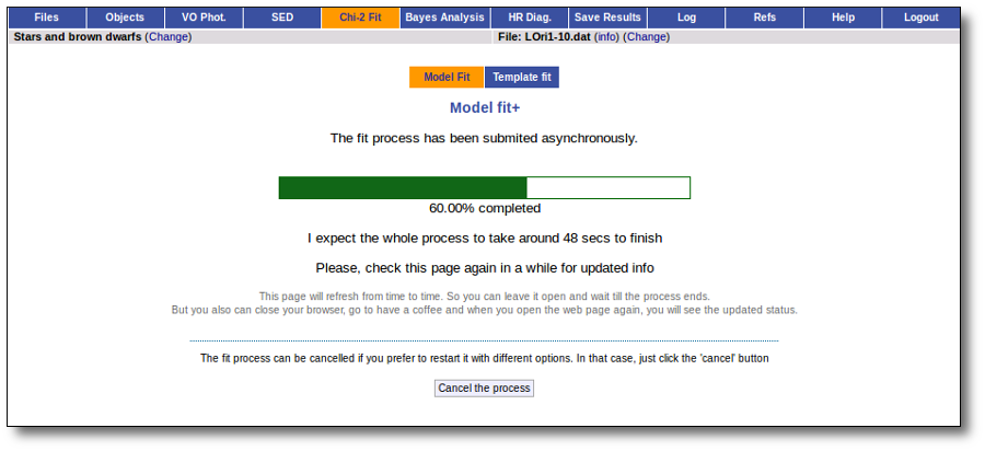
The fit process is performed asynchronously so that you don't need to stay in front of the computer waiting for the search results. You can close your browser and come back later. If the fit is not finished, VOSA will give you some estimation of the status of the operation and the remaining time.
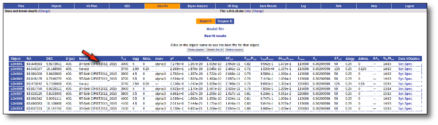
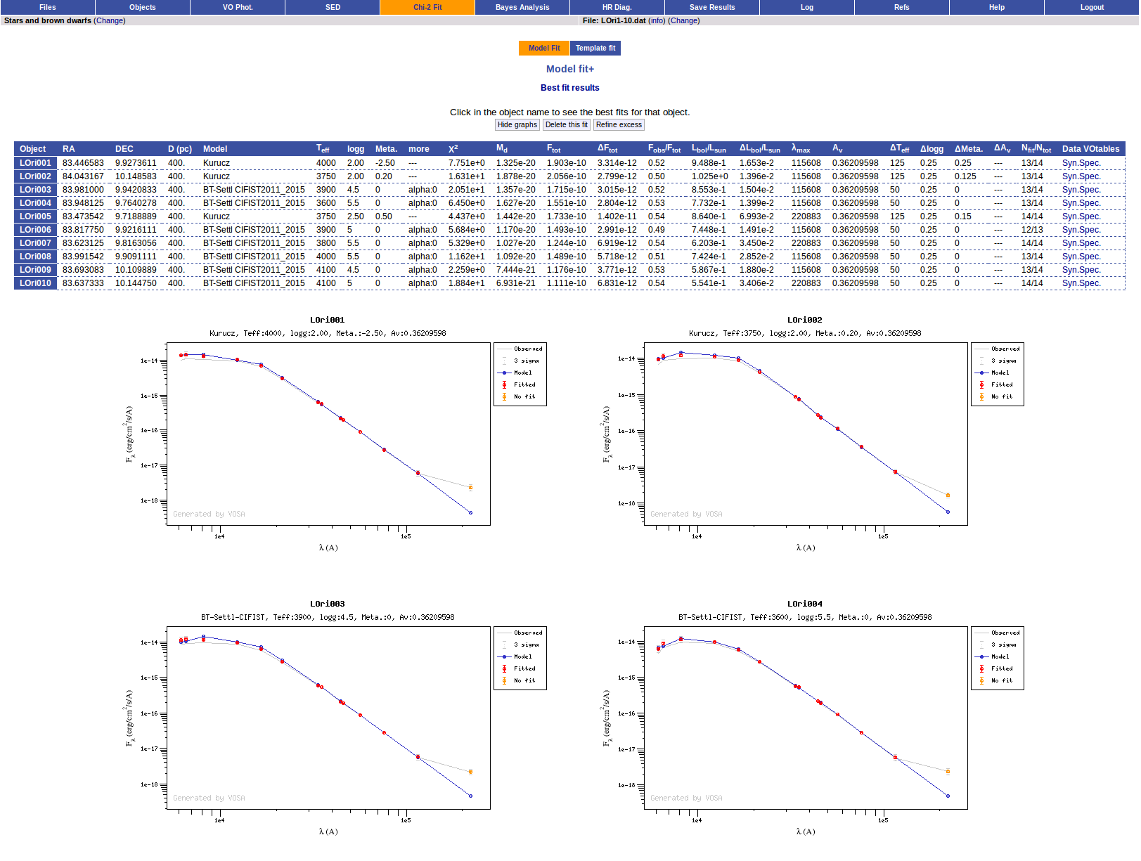
When the process finishes VOSA shows us a list with the best fit model (that is, the one with a smaller value for the reduced chi-2) for each object. Optionally you can also see the best fit plots, with the observed SED and the corresponding synthetic photometry for the best fit model.
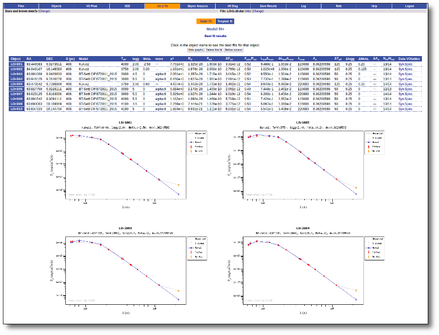 
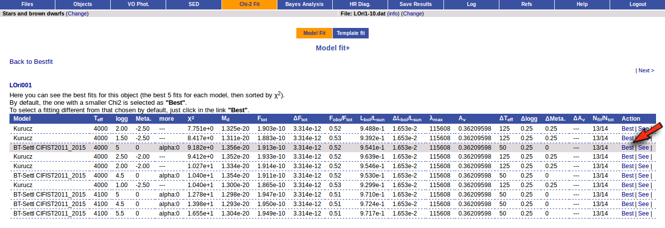
If you click one object name, you can see the 5 best fits for each collection of models. And clicking on the "See" link on the right of each fit, you can see the details about it.

Sometimes the fit with the best Χ2 is not the one that the user considers the best one, maybe for physical reasons, taking into account the obtained values of the parameters, or maybe because one prefers a model that fits better some of the points even having a larger Χ2... Whatever the reason, we have the option to mark as Best the model that we prefer. In order to do that we just click in the Best link at the right of the model that we prefer. In this case we choose the third one for LOri001.
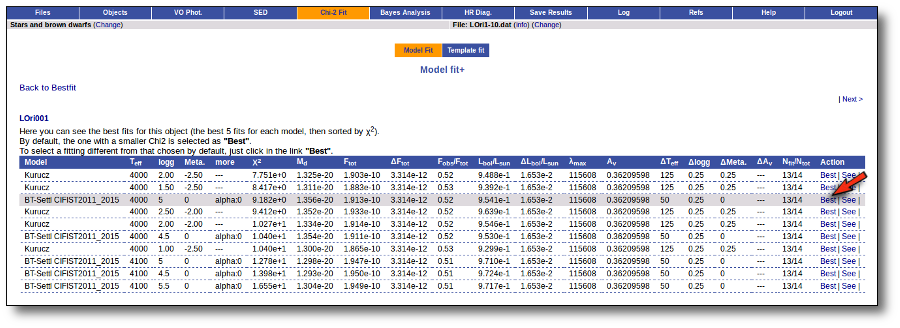
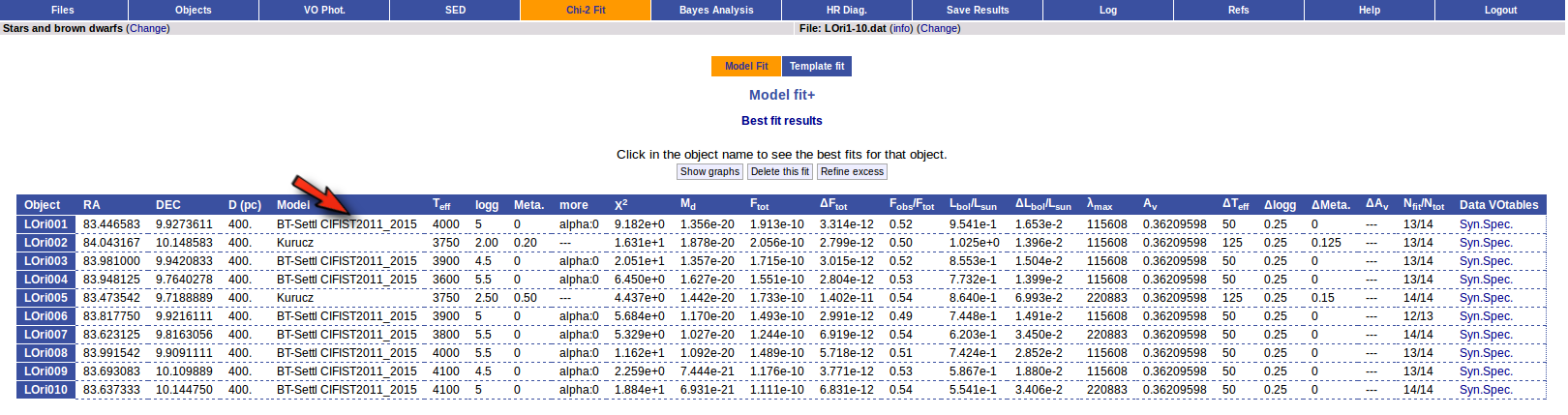
And when we go back to the bestfit list, we see that the fit that we have just selected is listed as the best one for LOri001.
At any time, you can move your mouse over each of the table headers and a window will appear with short explanation of the concept represented in that column.
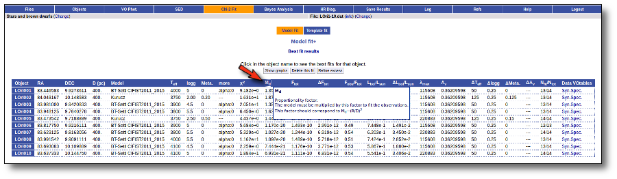
In this process we have been able to estimate some physical parameters for our objects. The models have given us the effective temperature, surface gravity and metallicity. Also, the total flux of the objects can be estimated using the model for those areas of the spectrum not covered by the observed photometry. And finally, using the distance given by user, the application estimates the bolometric luminosity of the object.
| Object |
Teff |
Log(G) |
Meta. |
Ftot |
Lbol/Lsun |
| LOri001 | 4000 | 5.0 | 0.0 | 1.913e-10 ± 3.314e-12 | 0.9541 ± 0.01653 |
| LOri002 | 3750 | 2.0 | 0.2 | 2.056e-10 ± 2.799e-12 | 1.025 ± 0.01396 |
| LOri003 | 3900 | 4.5 | 0.0 | 1.715e-10 ± 3.015e-12 | 0.8553 ± 0.01504 |
| LOri004 | 3600 | 5.5 | 0.0 | 1.551e-10 ± 2.804e-12 | 0.7732 ± 0.01399 |
| LOri005 | 3750 | 2.5 | 0.5 | 1.733e-10 ± 1.402e-11 | 0.864 ± 0.06993 |
| LOri006 | 3900 | 5.0 | 0.0 | 1.493e-10 ± 2.991e-12 | 0.7448 ± 0.01491 |
| LOri007 | 3800 | 5.5 | 0.0 | 1.244e-10 ± 6.919e-12 | 0.6203 ± 0.0345 |
| LOri008 | 4000 | 5.5 | 0.0 | 1.489e-10 ± 5.718e-12 | 0.7424 ± 0.02852 |
| LOri009 | 4100 | 4.5 | 0.0 | 1.176e-10 ± 3.771e-12 | 0.5867 ± 0.0188 |
| LOri010 | 4100 | 5.0 | 0.0 | 1.111e-10 ± 6.831e-12 | 0.5541 ± 0.03406 |
| 


 FAQ
FAQ