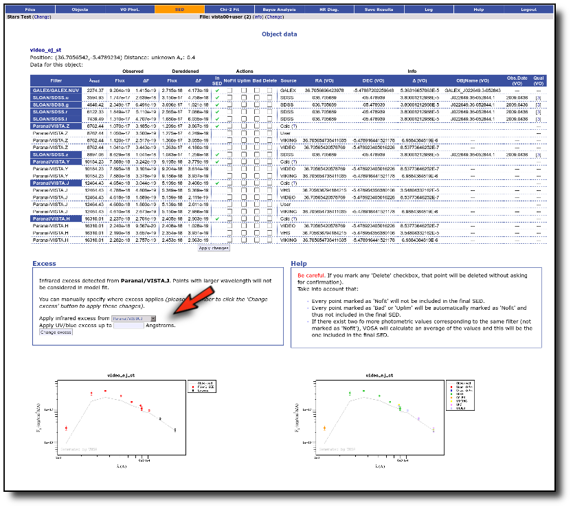
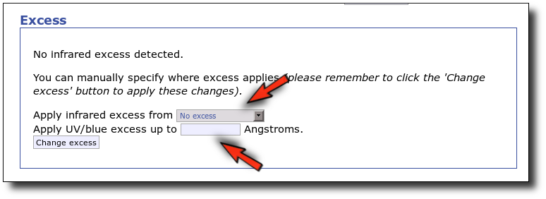
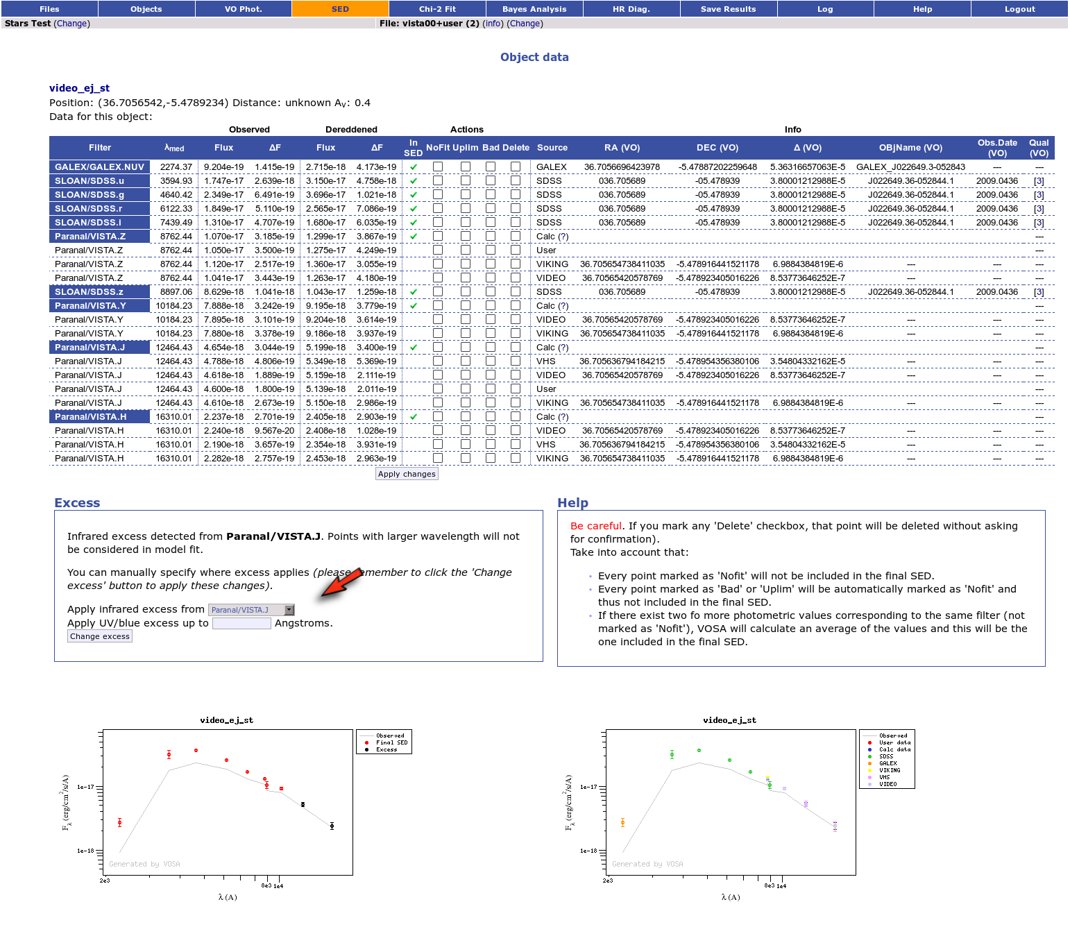
Excess

Most of the models used by VOSA for the analysis of the observed SEDs include only a photospheric contribution.

But the observed SED for some objects can include the contribution not only from the stellar photosphere but also from other components as disks or dust shells.

In these cases, some excess will appear and using the full SED for the analysis can be misleading.

Thus, VOSA offers the option to mark some part of the SED as "UV/Blue excess" or "Infrared excess" so that the corresponding points are not considered when the SED is analyzed using photospheric stellar models.

Infrared excess

VOSA tries to automatically detect possible infrared excesses.

Since most theoretical spectra used by VOSA correspond to stellar atmospheres only, for the calculation of the Χ_r² in the 'model fit' the tool only considers those data points of the SED corresponding to bluer wavelengths than the one where the excess has been flagged.

(Some models, as the GRAMS ones, include other components as dust shells around the star. For those cases the points marked as 'infrared excess' will be also considered in the model fit).

The last wavelength considered in the fitting process and the ratio between the total number of points belonging to the SED and those really used are displayed in the results tables.

The point where infrared excess starts is calculated, for each object, when you upload an input file, but it is also recalculated whenever the observed SED changes, that is:

• When VO photometry is added to the SED.
• When you delete a point in the SED or change something in the "SED" tab.

The excesses are detected by an algorithm based on calculating iteratively in the mid-infrared (adding a new data point from the SED at a time) the α parameter from Lada et al. (2006) (which becomes larger than -2.56 when the source presents an infrared excess). The actual algorithm used by VOSA is somewhat more sophisticated. A more detailed explanation is given below.

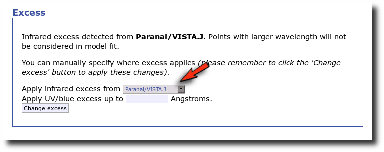
Apart from the automatic estimation made by VOSA, you can override this value specifying manually the point where infrared excess starts (so that more or less points are taken into account in the model fit) using the SED tab. Take into account that if you change the SED later (adding VO photometry or deleting a photometric point) this value will be recalculated again by VOSA.

It is also possible to specify the point where infrared excess start, for each object, as an 'object option' (10th column) in your input file. If you want to do this you have to include 'excfil:FilterName' (for instance: excfil:Spitzer/IRAC.I1) in the 10th column of the file. If you do that VOSA will not calculate the infrared excess for this object on upload and will accept the value given in the input file. But take into account that, if you change the SED later (adding VO photometry or deleting a photometric point) VOSA will recalculate the value even in this case.

Finally, you also have the possibility of changing the point where infrared excess starts for all objects at the same time. In order to do that, go to the SED tab and look for the "excess" link in the left menu. Once there, you have a form where this can be done.

IR excess automatic detection algorithm

The main idea is calculating, point by point in the infrared, the slope of the regression of the log-log curve showing $\nu F_{\nu}$ vs. $\nu$. At a first approximation, when this slope becomes smaller than 2.56, infrared excess starts.

In what follows, when we talk about regressions, we mean the regression of $y=log(\nu F_{\nu})$ as a function of $x=log(\nu)$, and taking into account observational errors as a weight for the regression. From error propagation, the "y" errors can be calculated as $\sigma(y) = \sigma(F_{\lambda})/(\ln10 F_{\lambda})$.

In order to avoid false detections due to "bad" photometric points, we refine the procedure as follows:

• We start at the first photometric point with $\lambda > 21500 A$.
• Points labeled as "nofit" are not considered in the algorithm.
• For each point (but the first one) we calculate:
  • The linear regression of all the points from the first to this one (without taking into account those already labeled as "excess suspicious", see bellow).
  • The $y$ value that would correspond to this point for a straight line starting on the first point and with slope=2.56. We call it $y_{\rm L}$.
• We mark the point as "excess suspicious" if it matches both of the following two criteria:
  • The regression slope (b), plus the error in the slope, is smaller than 2.56, that is: $$b+\sigma(b) < 2.56 $$
  • The observed value of $y$ is at least $3\sigma$ above the one predicted by the line with slope 2.56, that is: $$(y_{\rm obs} - y_{\rm L} ) > 3 \sigma(y)$$
• Points marked as "suspicious" will not be taken into account in further regressions.
• If two consecutive points are "suspicious" then VOSA marks the first of those points as the beginning of infrared excess.
• If one pointis suspcious and the next one isn't, then nothing happens. The first point (the suspicious one) will not be taken into account in further regressions, but we continue inspecting the next points.
• If the last point in the SED is suspicious, i.e., it matches both excess criteria, then that point is considered the beginning of inrrared excess even though the previous one did not match the criteria.

Apart from this, one more final criterium is applied. The slope (calculated as explained above) for at least one of the last two points in the SED must be sigma-compatible with being smaller than 2.56. $$b-\sigma(b) < 2.56$$

If this does not happen for any of the last two points, then there is no excess in the SED. The idea is that, if the infrared excess starts in some point it must continue for larger wavelengths. If that does not happen, any previous apparent detection of excess will be probably due to some "evil" combination of misleading points. In summary:

• The slope for at least one of the last two points in the sed must fulfill: $$b-\sigma(b) < 2.56$$
• two consecutive points must fulfill: $$b+\sigma(b) < 2.56 $$ $$(y_{\rm obs} - y_{\rm L} ) > 3 \sigma(y)$$ and then the infrared excess starts at the first of the two points.
• Or, if the last point in the SED meets those two criteria, even if the previous didn't, then the excess starts at the last point.

In the "Save Results", the user will be able to download files with a summary of the excess determination and with the details of each linear regression. These summary and details can also be visualized in the "SED" tab.

You can see some detailed examples of these calculations.

Fit refinement of the IR excess

When a model fit is completed, VOSA compares the observed SED with the best fit model synthetic photometry and makes a try to redefine the start of infrared excess as the point where the observed photometry starts being clearly above the model.

The procedure is as follows:

• If there is a point previously marked as the start of infrared excess VOSA starts the checking at that point.
• If not, VOSA starts in the medium point among those with λ > 21500A.
• For each point, VOSA checks for two criteria: $$\frac{F_{obs}-F_{mod}}{\Delta F_{obs}} > 3$$ $$\frac{F_{obs}-F_{mod}}{F_{mod}} > 0.2$$ that is, in plain words: the observation must be above the model, at least at a 3σ level, and the difference between both must be "significant".
• Both criteria must be fulfilled to consider that a point has excess (unless $\Delta F_{obs}=0$, that only the second crterium can be applied).
• If the criteria are fulfilled at the first point (thus, suspicious of 'fit excess') we check the previous point (smaller wavelength) and continue till one point doesn't match the criteria.
• If the criteria are NOT fulfilled at the first point (thus, no 'fit excess' detected) we check the next point (bigger wavelength) and continue till one point matches the criteria.

Let's see some examples.

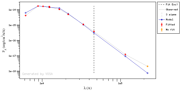
In the next case, when comparing the observed photometry with the model, VOSA sugests that the real infrared excess starts later than when the automatic algorith had detected:

In this image, looking at the fit, there is no apparent infrared excess (although the automatic algorithm had detected it):

In the following case, according to the "fit excess" criteria there is no infrared excess. This is due to the big observational errors. Instead, the automatic algorithm had detected it:

Onthe other hand, there are cases where the automatic detection algorith had not detected infrared excess but according to the fit, we see some excess:

And, obviously, in many cases both algorithms give the same result:

If for some objects the IR excess starting point calculated in this way is different from the one previosly calculated by the automatic algorithm, VOSA offers you the option to "Refine excess". If you click the corresponding button you will see the list of objects where this happens, the filters where excess starts according to both algorithms for each case, and the possibility of marking the start of infrared excess in the point flagged by the fit refinement instead of the one previously calculated by VOSA. If you choose to do this, and given that this would change the number of points actually used in the fit for those objects, the fit results are deleted and you have to restart the fit process. But, in what follows, the IR starting point will be the one suggested by the previous fit.

UV/blue excess

In some cases, there is also some excess in the bluer (UV) part of the SED.

VOSA does not detect this automatically, but you can specify it so that the application does not consider these points in the fits either.

The UV/blue excess can be set in two different ways:

• Including it in the input file as an 'object option' with the syntax Veil:VALUE, where VALUE is the value in Angstroms of the last wavelength where UV excess applies. For instance, if you include Veil:6000 in the 10th column of your input file for a given object, all the points with λ<=6000A will be marked as "Blue excess" and they will not considered in the fits.
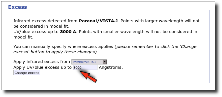
• Specifying this value manually in the SED tab.

Finally, you also can specify the same UV/blue excess range for all objects at the same time. In order to do that, go to the SED tab and look for the "excess" link in the left menu. Once there, you have a form where this can be done.

This Blue excess, as it happens with the infrared one, will not be taken into account for models that include not photospheric components (as the GRAMS ones).

An example

We are going to consider three different examples.

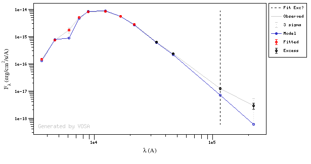
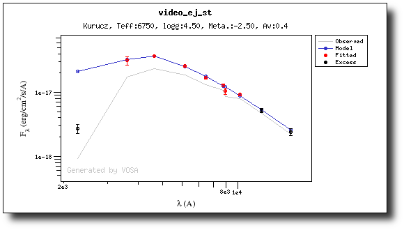
(1) Infrared excess only

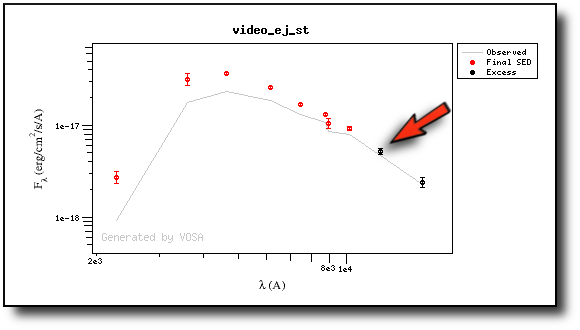
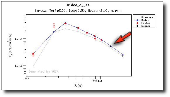
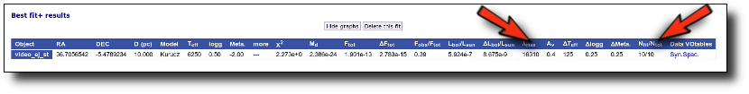
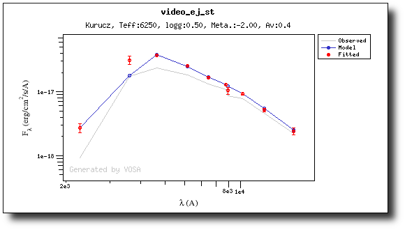
First, we leave the excess as detected by VOSA, starting at VISTA.J.

Those points are plotted in black in the SED.

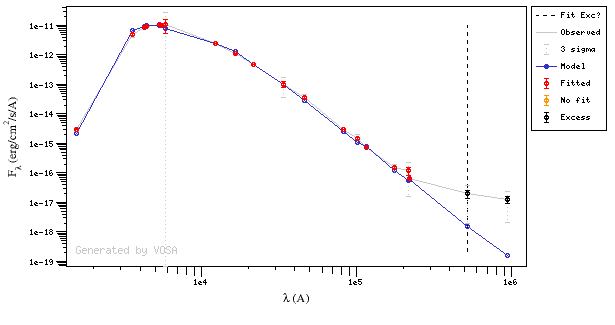
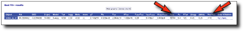
If we make a model fit for this object, the last two points in the SED won't be used. We see, in the results table, that only 8 of the 10 points have been used, and the wavelength of the last point fitted in the SED is the one for VISTA.J

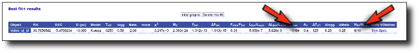
And these two points are shown in black also in the fit plot.

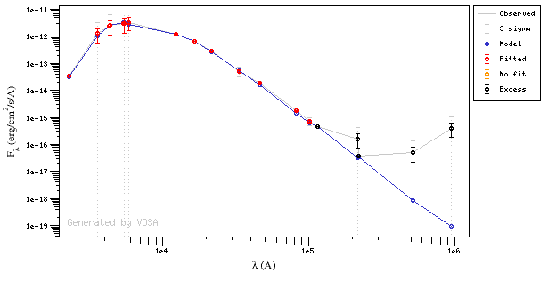
(2) Both UV/blue and infrared excess

Now we decide to go back to the SED tab and we make a change:

• There is also some UV/blue excess up to 3000A (so that the GALEX.NUV point will not be considered for the fit either).

This changes the SED plot accordingly.

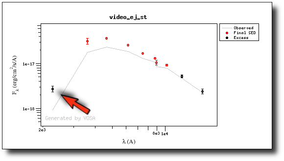
And when we repeat the model fit, the points that are fitted are only those that doesn't have excess now.

Actually, the best fit model is now a different one.

And the points in black in the fit plot are the ones corresponding to the excess that we specified manually (the GALEX.NUV point is not taken into account for the fit).

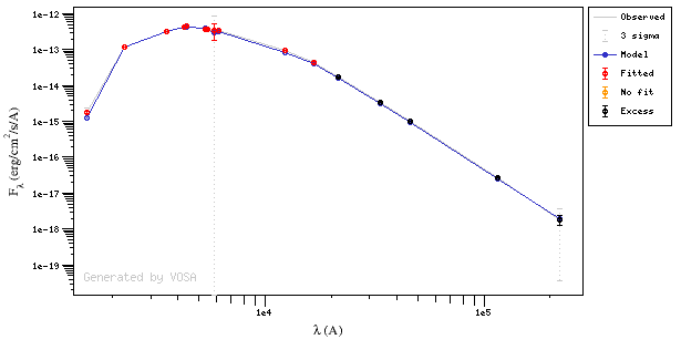
(3) No excess

As a last example, we go back to the SED tab and set that there is no infrared or UV/blue excess.

This changes the SED plot accordingly.

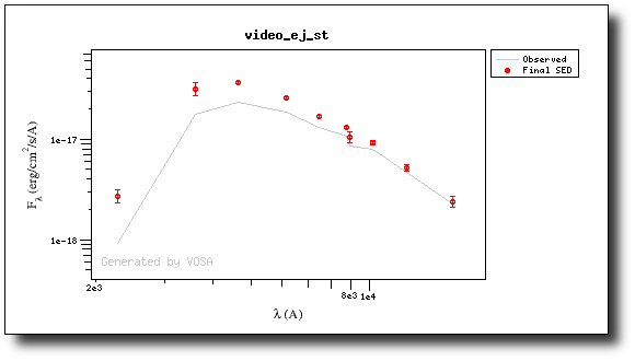
And when we repeat the model fit, all the points are considered for the fit now.

And all the points are shown in ref (fitted) in the plot.

SED

Model Fit