Bayes analysis

While the chi-square fit gives the best fit model for each object, the Bayesian analysis provides the projected probability distribution functions (PDFs) for each parameter of the grid of synthetic spectra.

The procedure followed by VOSA to perform a Bayesian analysis of the model fit is as follows:

• We first calculate a $\chi^2$ model fit as explained in [Model fit] .

• Then we assign a relative probability for each model as: $$W_i = \exp(-\chi_i^2/2)$$

• Using this, the probability corresponding to a given parameter value $\alpha_j$ is given by: $$P(\alpha_j) = \sum_i W_i$$

  where the sum is performed over all the models with that value for that parameter.

• We finally normalize these probabilities, for each parameter, dividing by the total probability (the sum of the probilities obtained for each value). $$P'(\alpha_j) = \frac{P(\alpha_j)}{\sum_i P(\alpha_i)}$$

In the case that you have decided to consider Av as a fit parameter (giving a range of Av values to try), the probability distribution for Av is calculated too.

Example

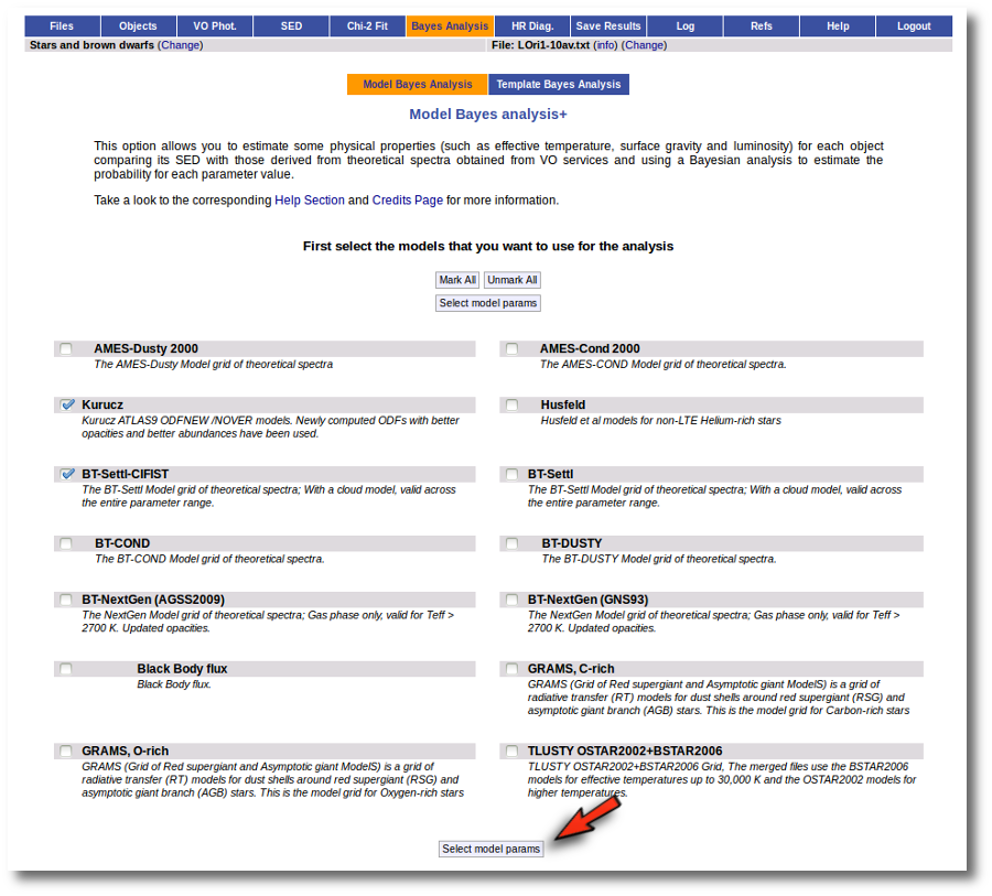
We enter the "Model Bayes Analysis" tab and we see a form with the available theoretical models, so that we can choose what ones we want to use in the fit. In this case we decide to try Kurucz and BT-Settl-CIFIST models. Thus, we mark them and click in the "Next: Select model params" button.

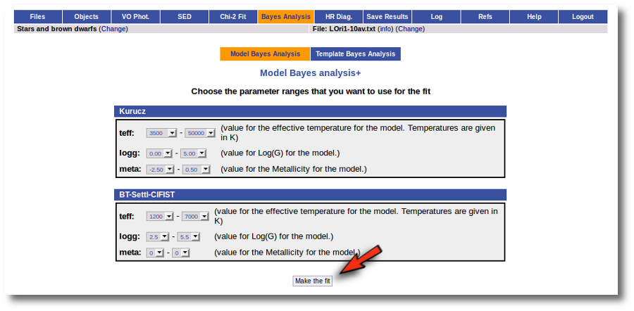
For each of the models, we see a form with the parameters for each model and the available range of values for each of them. In this case we are going to try the full range of parameters, so we leave the form as it is and then click the "Next: Make the fit" button.

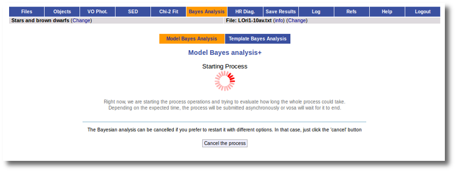
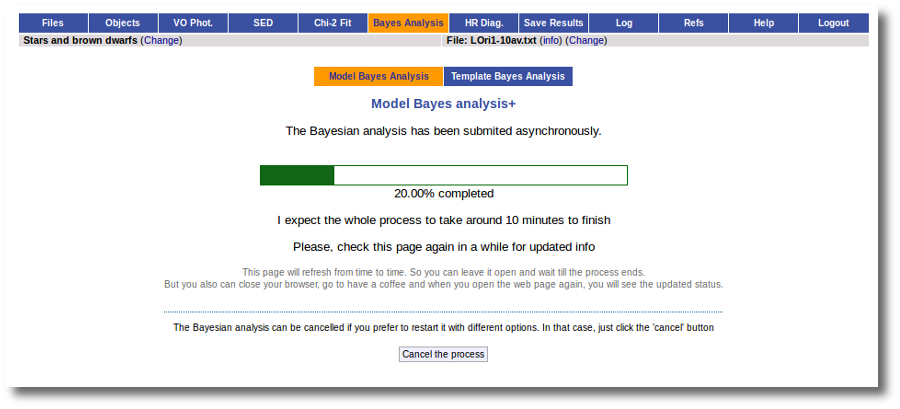
In this case, VOSA will have to calculate the chi-square fits and then use them to perform the analysis. The fit and analysis process is performed asynchronously so that you don't need to stay in front of the computer waiting for the search results. You can close your browser and come back later. If the process is not finished, VOSA will give you some estimation of the status of the operation and the remaining time.

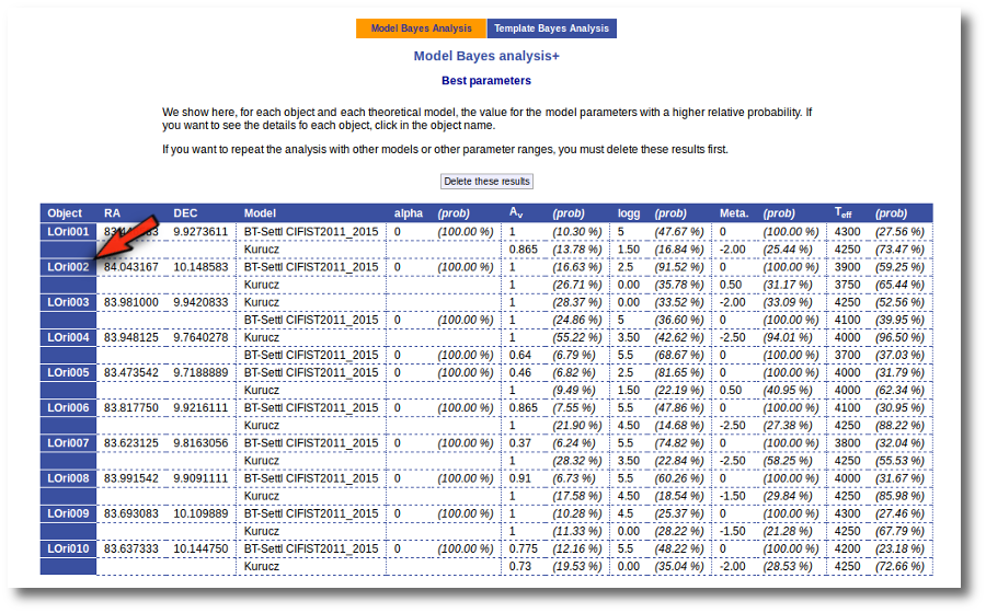
When the process finishes VOSA shows us a list with, for each object and each model collection, the most probable value for each parameter and its probability.

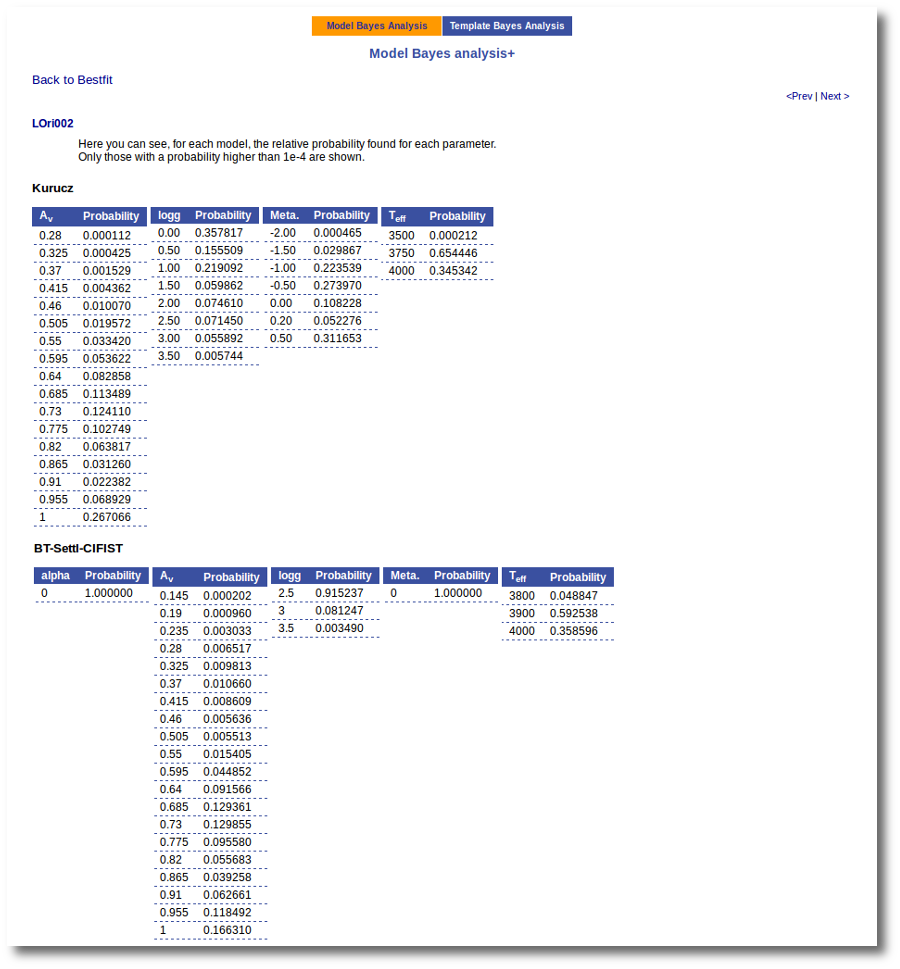
And if we click in one of the object names, we can see all the details of the analysis for this object.

We see first the probability of each value of each model parameter (only those values with a non-negligible probability are shown).

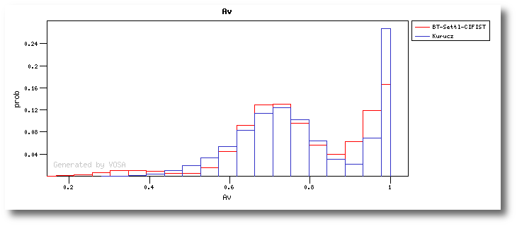
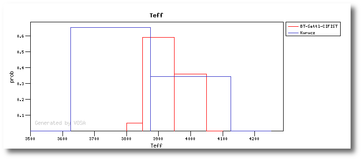
And then some simple plots of these probability distributions.

Model Fit

Template Fit