HR diagram

VOSA offers the option to estimate values for the age and the mass of the objects. In order to do that, the (T_eff,log(L)) values obtained from the chi-square fit are used as starting points for interpolating collections of theoretical isochrones and evolutionary tracks obtained from the VO. Then, a HR diagram is displayed showing the data points, isochrones and evolutionary tracks.

For each object, only the theoretical isochrones and evolutionary tracks more adequate to the model that best fits the observed photometry are used in the process. For instance, in the case where this model is "Kurucz" the Siess isochrones are used.

In the case that several collections are used (because we use one for some objects and another one for other objects) a HR plot will be generated for each collection, showing the isochrones, tracks and the points corresponding to the objects analysed using that collection.

You can play with the plots, decide to plot more or less information, locate the objects in it, etc.

Error estimation

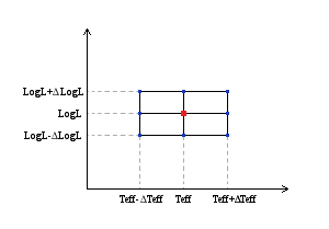
In order to make an error estimation, the errors coming from the chi-square fit for T_eff and LogL are used to generate a small grid with 9 points.

For each of these 9 points we make the interpolation as explained below.

The final values for (Age,Mass) will be the ones obtained for the point (Teff,LogL). But in some cases, the interpolated value of Age or Mass is different for some of the other 8 points. Thus, in the results table we show the minimum and maximum value obtained for each parameter when using any of the 9 points in this small grid.

Interpolation

(Below, all the explanations are given for the case of obtaining an estimation of the object age interpolating on isochrones. Everything is valid also for the case of obtaining an estimation of the mass interpolating on evolutionary tracks.)

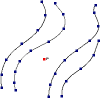
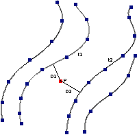
The interpolation between isochrones involves to find the two closer isochrones to the (T_eff,log(L)) point (one to each side of the point), calculate the distance from the point to each of the curves and, then evaluate a weighted average between the values of t for each isochrone.

$t=\frac{t_2 D_1+t_1 D_2}{D_1+D_2}$

In order to do this it is necessary to design an algorithm able to estimate the distance from a point to a curve defined by discrete points (note that we do not have an analytical curve but just a series of points that are assumed to define a curve).

Distance from a point to a curve

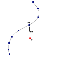
1.-The main method that we use to estimate the distance form the point to an isochrone is as follows:

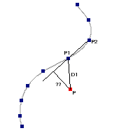
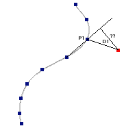
• First, given the point P (T_eff,log(L)) find the closest point in the curve (point P1 at a distance D1)
• Second, find the projection of P to the line defined by P1 and either the next point in the curve or the prior one.
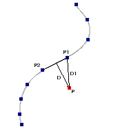
• If either of the projections lies into the interval defined by the two points (P1 and P2), then calculate the distance from the point P to the projection.
• This value will be taken as the distance from P to the isochrone.

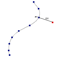
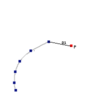
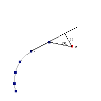
2.-In some cases, it is not possible to use the above method because none of the proyections lie inside the interval between the two points that define the line.

When that is the case, we can estimate the distance to the curve as the distance D1 from P to the closest point in the curve P1

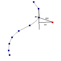
Note that we consider this a worse approximation in general. Actually it is highly probable to be bad when P1 is the fist or last point in the curve.

That is why we this method will only be used if the first one fails and if the closest point P1 is not the fist or last point in the curve.

Interpolated value for the age

If we have been able to find a curve on each side of the point P and the distance from that point to each curve, we can use the inverse of the distance as weights: $$t=\frac{\frac{1}{D_1}t_1+\frac{1}{D_2}t_2}{\frac{1}{D_1}+\frac{1}{D_2}}=\frac{t_2 D_1+t_1 D_2}{D_1+D_2}$$

In some cases, we are able to determine only the distance to one curve, but we know that there exist an isochrone on each side of the point. If that happens we just show a range of values for the age using the ones corresponding to each isochrone as lower and upper limits.

Finally, if the point lies outside the area covered by the isochrones, we do not even try to estimate a value for the age or the mass of the object.

Flags for interpolated values

Whenever we are not able to find a value for the age or the mass of an object or it has been determined using a worse approximation that the one that we consider the best (See above) a flag is shown right to the value.

These are the possible flags and their meanings:

Example

We have made a chi-square model fit for a set of objects. The best fit model for all the objects was BT-Settl-CIFIST. Thus, when we enter the "HR diagram" tab we see the collection of isochrones and tracks that is going to be used as default for all the objects: BHAC15.

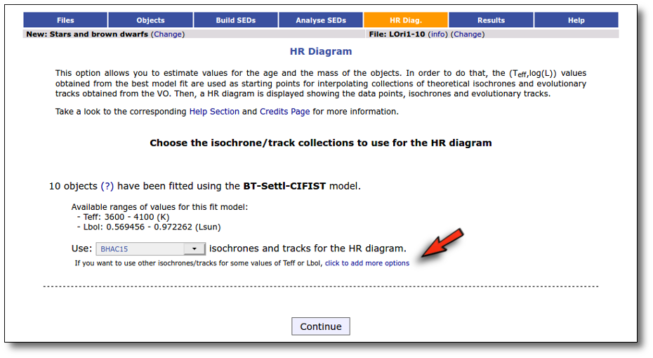
But we can click in the "click to add more options" link to change the default behaviour.

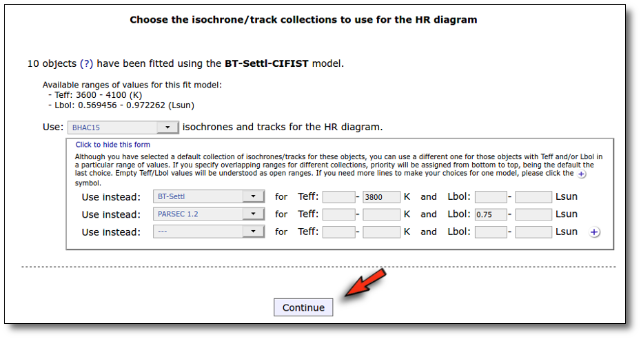
When we click the link a new form opens that allows to choose different isochrones/tracks collections depending on the Teff and Lbol values of each object. For instance, in this case we configure:

• Use BT-Settl isochrones/tracks if Teff < 3800K.
• Use Parsec 1.2 isochrones/tracks if Lbol > 0.75 Lsun.
• BHAC15 isochrones/tracks will be used for those objects that don't meet any of those conditions.

Take into account that if some object meets several conditions (for instance, Teff<=3800K and Lbol >= 0.75) priority will be assigned from bottom to top, being the default the last choice (that is, in this case, Parsec 1.2 will be used).

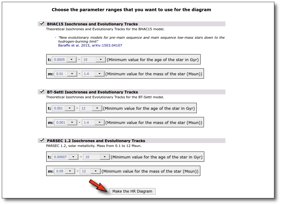
When we click the "Continue" button, we will see the available ranges of values (age and mass) available for each of the choosen collections. We could play with the ranges of parameters, restricting the values of the age and mass to be considered in the analysis. But we prefer to keep the full range and click the "Make the HR Diagram" button.

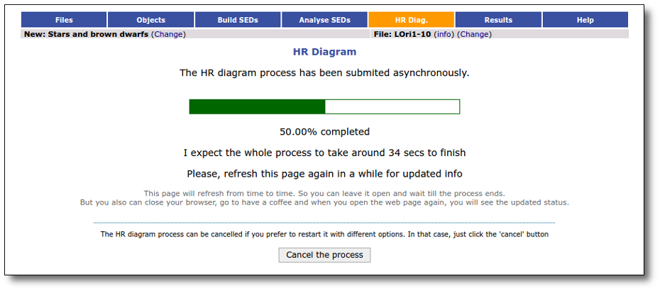
The interpolation process, to obtain the best values (and ranges) for the age and mass of each object, is performed asynchronously so that you don't need to stay in front of the computer waiting for the results. You can close your browser and come back later. If the process is not finished, VOSA will give you some estimation of the status of the operation and the remaining time.

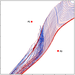
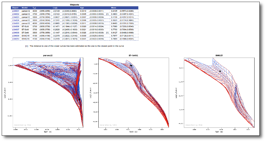
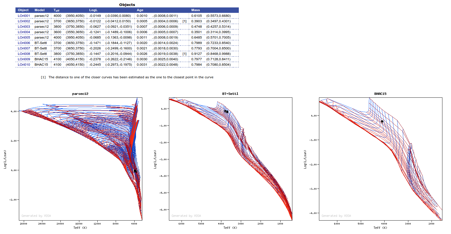
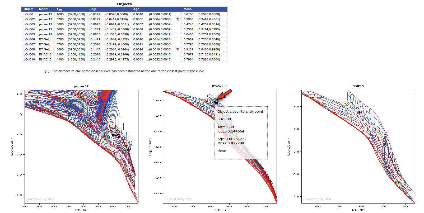
When the process is finished, you can see the list of objects with the interpolation results, and three HR plots, one for each collection of isochrones and tracks.

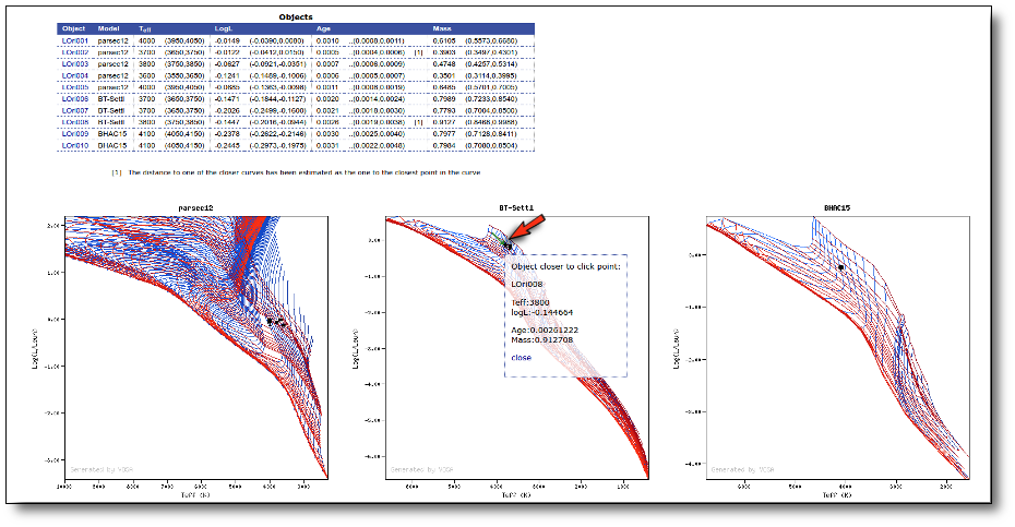
If you click in any graph, VOSA will locate the object closest to the click point and will show you its properties.

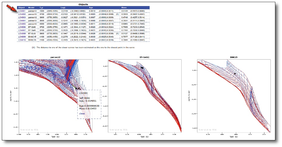
If, instead, you click on one object name in the list, VOSA will locate that object in the corresponding graph.

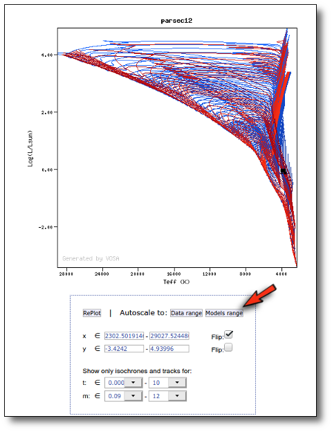
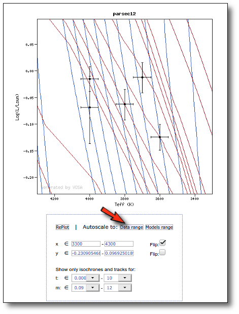
You also can play with the plots. There are options to zoom to the objects range or to the models range. Other options allow you to define the exact range of each coordinate. And you also can decide what isochrones or tracks you want to display.

Binary Fit

Upper Limits