FAQ
Distances
Why parallax errors in TGAS are larger in VOSA than those given by the catalogue?
VOSA adds a sistematic error of 0.3 mas to the original error, as recommended in Brown et al. 2016.
Catalogs / Photometry
How is the counterpart selected in the photometric catalogs?
We always take the nearest counterpart within the search radius chosen
in the "VO Photometry" tag. For those catalogues containing both point
and extended sources (e.g. SDSS, UKIDSS, VISTA, DES,...), if the nearest
counterpart is an extended object, then VOSA does not return any
photometric information.
If a photometric point has ΔFlux=0, how is this treated in the fit?
In summary, points with ΔFlux=0 are treated as if they had the largest error in the SED. VOSA calulates the largest relative error in the SED, adds a 10% and then assigns this relative error to those points without an observational ΔFlux. See the Fit help section for details.
From magnitudes to fluxes: How does VOSA compute the error in flux from the error in the catalogue magnitudes?
For pogson magnitudes, being ${\rm F}_0$ the photometric system zero point flux:
$${\rm mag} \pm \Delta {\rm mag} \Rightarrow {\rm Flx} \pm \Delta {\rm Flx}$$
$${\rm Flx} = {\rm F}_0 \ 10^{-{\rm mag}/2.5} $$
$$\Delta {\rm Flx} = {\rm Flx} \cdot \Delta {\rm mag} \cdot \ln(10)/2.5$$
Stromgren: Does Paunzen (2015; J/A+A/580/A23) supersede Hauck et al. (1997; II/215)?
No. They are different catalogues. The number of sources in common is less than 50% and Hauck et al. (1997) has even more sources than Paunzen (2015).
Stromgren: Why, sometimes, the errors in flux associated to the photometric values of the Paunzen catalogue are larger than the rest of photometric points?
There are two main reasons for this effect:
- Sometimes, the magnitude given by the catalogue is just the average of different measurements taken at different epochs by different groups. In this case the error in the magnitude is the standard deviation of these measurements which may be large in some occasions.
- Sometimes, magnitudes in the Paunzen catalogue have no associated errors. In this case, VOSA assigns to these magnitudes, in the chi2 process, the largest of the photometric errors multiplied by 1.1. If you visualize the SED in the chi2-fit tab, you will see these large asigned errors.
Stromgren: How do we go from the information available in Stromgren photometry catalogues (V, (b-y), m1, c1 and the respective errors) to the uvby magnitudes and the respective errors?
The catalog provides:
$$ V \pm \Delta V $$
$$ (b-y) \pm \Delta (b-y) $$
$$ m1 \pm \Delta m1 $$
$$ c1 \pm \Delta c1 $$
and we calculate:
$$ y = V $$
$$ b = (b-y) + y $$
$$ v = m1 + 2(b-y) + y $$
$$ u = c1 + 2m1 + 3(b-y) + y $$
$$ \Delta y = \Delta V $$
$$ \Delta b = \sqrt{ \Delta (b-y)^2 + \Delta y^2 } $$
$$ \Delta v = \sqrt{ \Delta m1^2 + 4\Delta (b-y)^2 + \Delta y^2 } $$
$$ \Delta u = \sqrt{ \Delta c1^2 + 4 \Delta m1^2 + 9\Delta (b-y)^2 + \Delta y^2 } $$
Which catalogues are included in the "info/refs.dat",
"info/refs.bibtex.bib" files, automatically generated when the results
are downloaded?
References of all used catalogues can be downloaded from the "Download
Results" tab. In the case of photometric catalogues in which a
counterpart to the target exists, They will be included in the
"info/refs.dat", "info/refs.bibtex.bib" files, regardless the
utilization of these points to build the SED.
On the contrary, if the target has no counterpart in a catalogue, this
catalogue will not be included in those files.
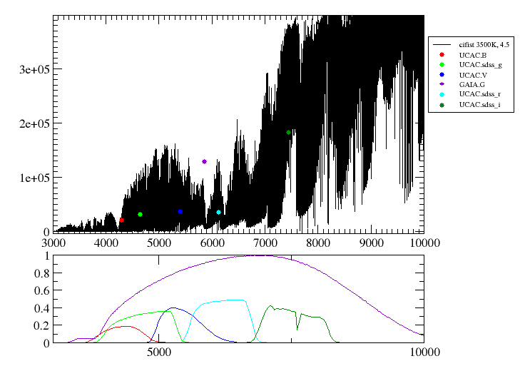
Why does Gaia photometry appear to be clearly outside the SED even for good fits?
The fact is that Gaia G filter is very wide compared to most filters with similar wavelegths. Thus, it averages the spectrum over a large wavelenth range. If it happens that the spectrum is steppy in that range, the photometric point will typically lie far from the spectrum and probably outside the main SED tendency.
This is just an example of the fact that you shouldn't try to fit observed photometry using the theoretical spectrum directly. You need to compare the observed photometry with the synthetic one calculated using the theoretical spectra and the filter passband.
Why does it happen that, in particular cases, SDSS fluxes are negative?
Magnitudes should not produce negative fluxes but SDSS magnitudes are not the typical pogson ones but asinh "laptitudes" and the conversion formula that we apply is:
$${\rm Flx} = {\rm F}_0 \ 10^{-{\rm mag}/2.5} [ 1-{\rm b}^2 * 10^{2 {\rm mag}/2.5}]$$
this shouldn't produce negative fluxes either but it can happen and, when it happens, VOSA rejects the corresponding flux values as bad.
You can take a look to the filter information for more details and the particular parameter values for each SDSS filter.
Model fit
The Av/Teff degeneracy: What is the combined effect of extinction and effective temperature in the SED?
If the precise value of Av is not known and you choose to include it as a fit parameter, and specially when no photometric information in the blue range is available, it may happen that different combinations of extincion and effective temperature give very similar fits leading to a Av/Teff degeneracy.
This effect is considerably reduced when the distance to the object is known so that you can restrict to small values of Av.
This can be clearly seen if the Bayes analysis is performed (see figures). In this case, the best effective temperature calculated using the chi2 fit may not be the good one from the physical point of view.
Why The fit process takes much longer when you decide to include the model spectrum in the fit plots?
Some theoretical spectra like, for instance, the BT-Settl-CIFIST ones, are very big files. If you decide to include the spectra in the plots, VOSA, during the processing of the fit results, has to ask the corresponding VO service for a degradated version of the best fit spectrum for each object. The VO service makes the calculation to degradate the spectrum, returns it to VOSA and VOSA includes it in the plot. This operation takes longer for big spectra (like BT-Settl-CIFIST), maybe a few seconds, but the acumulated time excess for many objects can be very relevant.
Thus, if you have a VOSA file with thousands of objects, don't check the "Include model spectrum in fit plots?" unless you really need that.
Output products
Why the theoretical models that best fit for each object (that is, already multiplied by Md and scaled to the observational points) are not included in the list of VOSA products, for instance as a lambda, flux table?
The theoretical spectra are not included in the list fo VOSA products mainly because of their size. For instance, the size of a single BT-Settl spectrum is 8 MB.
The best way to download the theoretical spectrum that best fits the data is going to the "Best fit" table of results. The last column of the table, titled "Data VOTables" gives you a link to get the full theoretical spectrum corresponding to each object fit.
WARNING: As these files may be large, and in order to avoid web browser crashes, it is advisable to save them using the "Save as" option (right buttom of the mouse) instead of directly cliking on the link.
Besides this, as a side trick, take into account that .agr files for the plots with the fit results contain a resampled version (lower resolution) of the theoretical spectrum if you have chosen to include spectra in the plots. These are ascii files, and you can find the spectrum at the end of the file as the table with the largest number of points.
| 
 Phys. Constants