Model Fit
One of the main analysis options of this application is the Model fit.
Here the observed SED for each object is compared to the synthetic photometry for several theoretical models using a chi-square test. This gives an estimate of the physical properties of the given object.
If you provide a range for the visual extinction (AV), this fitting will also consider it as a fit parameter, as explained below.
Fit
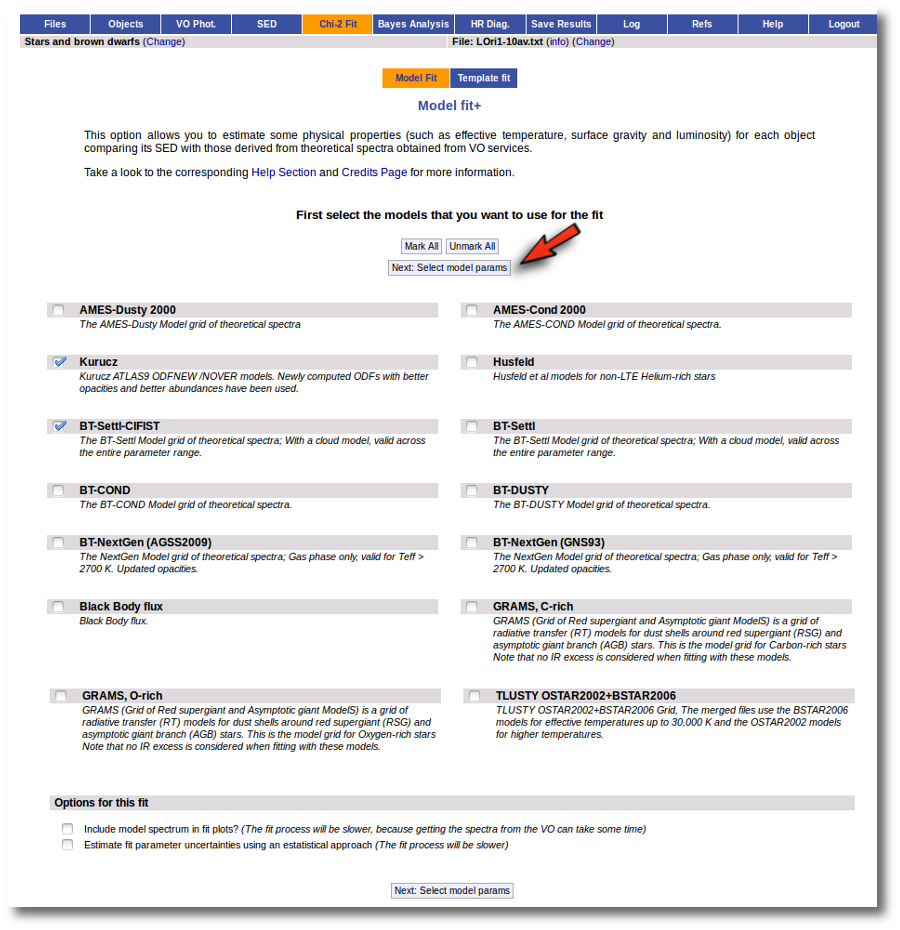
When a fitting process is started you can choose among a list of theoretical spectra models available in the VO. Only those that are checked will be used for the fit.
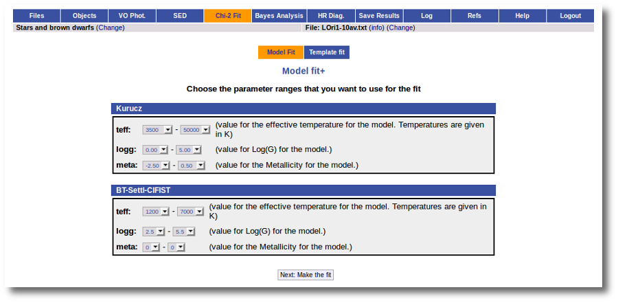
In the next step the application uses the TSAP protocol (SSAP for theoretical spectra) for asking the model servers which parameters are available to perform a search. According to that, a form is built for each model so that you can choose the ranges of parameters that you want to use for the fit. Take into account that:
- The fitting process implies queries to VO services, data sent through the network, a lot of calculations (some done by the services themselves and some done by the application)... That means that it could take a long time to get the final results.
- Using more models and wider ranges of parameters will imply a longer time for the fitting (specially if your file contains many objects) so be ready for a long waiting time in the next step.
- In some cases, the whole range of parameters offered by the models are not right for your objects. For instance, if you know, for whatever physical reasons, that your objects have small temperatures, choose only small temperatures in the forms to optimize the process.
- The response time has roughly linear dependence on the number of objects in the file (twice number of objects means twice waiting time). Thus, you could prefer splitting your input file in different ones (according to physical properties, pertenence to a group or other reasons) better than doing all the work in an only data file.
- If you decide to fit the extinction too (giving a range for AV) this will also increase the fitting time. Take into account that 20 different values of AV are considered for each object/model combination. Although this won't imply a fitting time 20 times larger, it also enlarges the calculation time.
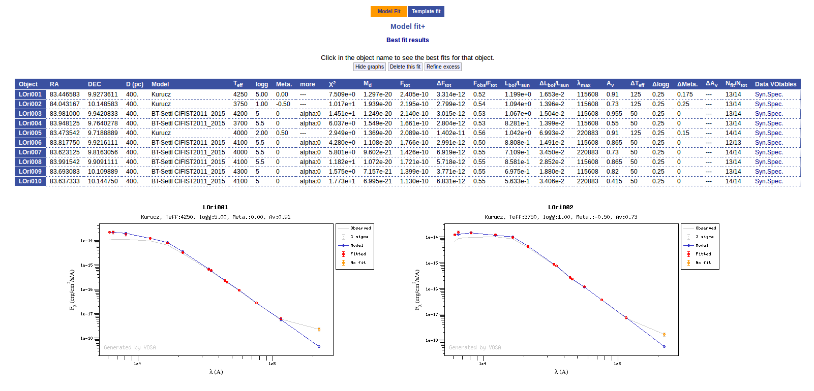
Once the fit has been finished, you can see a list with the best fit for each object and, optionally, a plot of these fits.
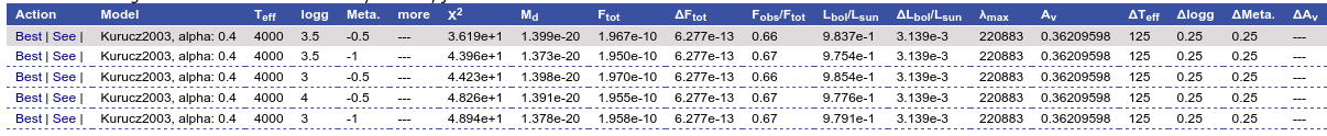
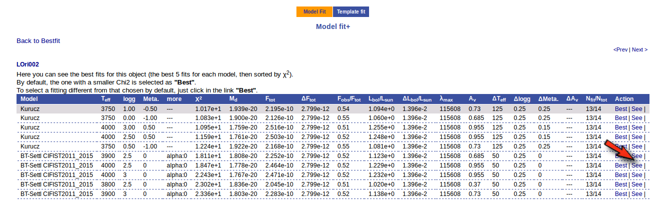
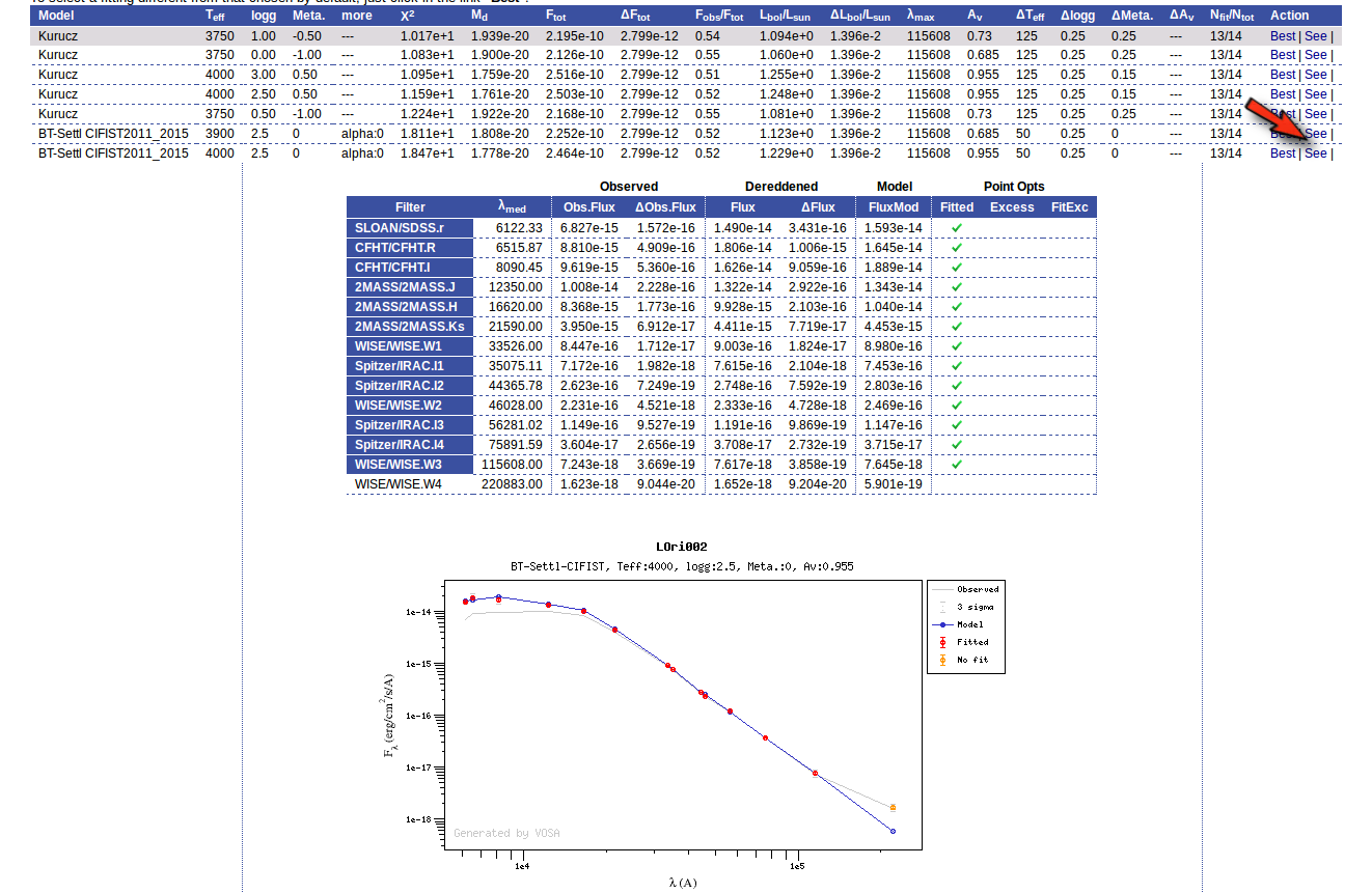
Besides that, for each particular object, you can also see a list with the best 5 fits for each model sorted by χ2. For each result you can see the corresponding SED and plot (with the "See" button) or use the "Best" button to mark a different result as the preferred best one. If you do that, this fit will be highlighted and it will be the one that will be shown in the "Best fit" table later.
Best Fit
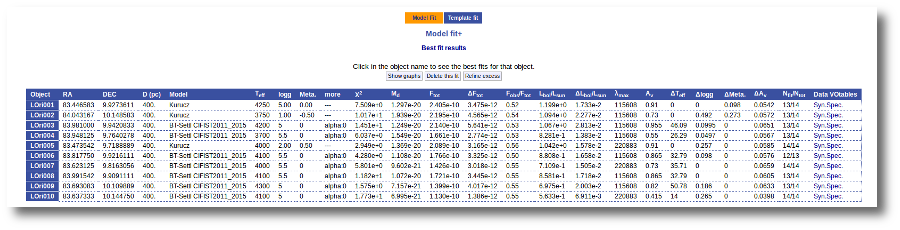
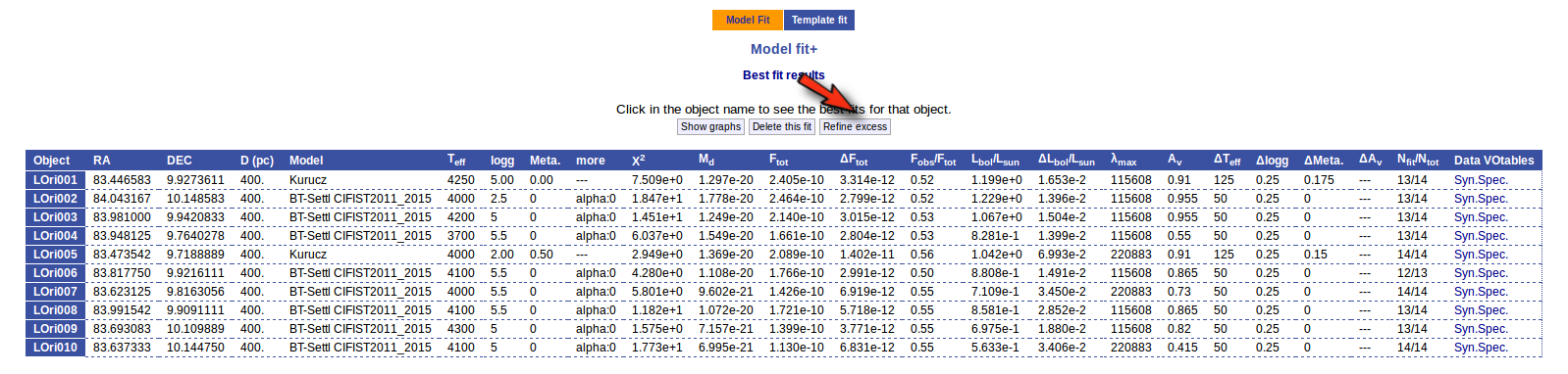
Once a fit has been done, you can see the Best Fit table with the best fit properties for each object.
A number of results are shown for each object:
- Object name, as given by the user.
- RA, Right Ascension as given by the user.
- DEC, Declination as given by the user.
- D(pc): distance in pc as given by the user (if the user does not provide a value, a typical default value of 10pc is used).
- Model name that best fits the data.
- Teff: effective temperature, in K, for the model that best fits the data.
- Log(G): logarithm of the gravity for the model that best fits the data.
- Metallicity: metallicity for the model that best fits the data.
- More: values for other (not so common) parameters used by the model.
- Χr2: value of the reduced chi-squared parameter for the fit (see below).
- Md: dilution factor. Value by which the model has to be multiplied to fit the data (see below).
- Ftot: Total flux (see below).
- ΔFtot: error for the total flux.
- Fobs/Ftot: fraction of the total flux obtained from the observed photometry (See below).
- Lbol/Lsun: Bolometric luminosity (See below).
- ΔLbol/Lsun: error for the Bolometric luminosity.
- λmax: value of the last wavelength considered for the fitting In order to avoid data with excess) (See below).
- AV: final value of AV used for dereddening the sed.
- ΔTeff: uncertainty for the effective temperature. It's estimated as half the grid step, around the given value, for this model.
- ΔLog(G): uncertainty for the logarithm of the gravity. It's estimated as half the grid step, around the given value, for this model.
- ΔMeta.: uncertainty for the metallicity. It's estimated as half the grid step, around the given value, for this model.
- ΔAV.: uncertainty in the value of AV (in the case that AV has been used as a fit parameter).
- R1. Estimate of the stellar radius obtained using Md and the distance (See below).
- ΔR1. Uncertainty on R1 (See below).
- R2. Estimate of the stellar radius obtained using logg and the distance (See below).
- ΔR2. Uncertainty on R2 (See below).
- M1. Estimate of the stellar Mass using Lbol and R1 (See below).
- ΔM1. Uncertainty on M1 (See below).
- M2. Estimate of the stellar Mass using Lbol and R2 (See below).
- ΔM2. Uncertainty on M2 (See below).
- Nfit/Ntot: Number of points considered in the fitting (not taking into account points with excess or points labeled as 'nofit') divided by the total number of observed points (See below).
- Link to a VOtable with the synthetic spectra corresponding to the best fit.
When the fit has been made with the option of calculating parameter uncertainties using a Monte Carlo method, a statistical distribution is obtained for these parameters and some other values are shown in this table:
- Teff,min,68, Teff,max,68: Minimum and maximum value for the effective temperature at the 68% confidence level. Calculated as the 14 and 84 percentiles of the distribution.
- Teff,min,96, Teff,max,96: Minimum and maximum value for the effective temperature at the 96% confidence level. Calculated as the 2 and 98 percentiles of the distribution.
- loggmin,68, loggmax,68: Minimum and maximum value for logg at the 68% confidence level. Calculated as the 14 and 84 percentiles of the distribution.
- loggmin,96, loggmax,96: Minimum and maximum value for logg at the 96% confidence level. Calculated as the 2 and 98 percentiles of the distribution.
- Metamin,68, Metamax,68: Minimum and maximum value for the Metallicity at the 68% confidence level. Calculated as the 14 and 84 percentiles of the distribution.
- Metamin,96, Metamax,96: Minimum and maximum value for the Metallicity at the 96% confidence level. Calculated as the 2 and 98 percentiles of the distribution.
- AV,min,68, AV,max,68: Minimum and maximum value for AV at the 68% confidence level. Calculated as the 14 and 84 percentiles of the distribution.
- AV,min,96, FV,max,96: Minimum and maximum value for AV at the 96% confidence level. Calculated as the 2 and 98 percentiles of the distribution.
- Ftot,min,68, Ftot,max,68: Minimum and maximum value for the total Flux at the 68% confidence level. Calculated as the 14 and 84 percentiles of the distribution.
- Ftot,min,96, Ftot,max,96: Minimum and maximum value for the total Flux at the 96% confidence level. Calculated as the 2 and 98 percentiles of the distribution.
Extinction fit
If a range for the visual extinction (AV) is given, it will also be considered a fit parameter.
You can provide this range for each object in two different ways:
- In the input file (10th column). See Upload file format section for more info.
- In the "Objects: extinction" tab.
If you don't provide a range for AV, the default value provided by you (also in the input file or the Extinction tab) will be used.
If you provide a range, like for instance AV:0.5/5.5, the fit service will compare each particular file of the model with the observed SED dereddened using 20 different values for AV in that range. Then the best fit models will be returned by the service with the best corresponding value of AV.
Reduced chi-square
The fit process minimizes the value of Χr2 defined as:
$$\chi_r^2=\frac{1}{N-n_p}\sum_{i=1}^N\left\{\frac{(Y_{i,o}-M_d Y_{i,m})^2}{\sigma_{i,o}^2}\right\}$$
Where:
| N: | Number of photometric points. |
| np: | Number of fitted parameters for the model.
(N-np are the degrees of freedom associated to the chi-square test) |
| Yo: | observed flux. |
| σo: | observational error in the flux. |
| Ym: | theoretical flux predicted by the model. |
| Md: | Multiplicative dilution factor, defined as: $M_d=(R/D)^2$,
being R the object radius and D the distance between the object and the observer.
It is calculated as a result of the fit too. |
Visual goodness of fit
Two extra parameters, Vgf and Vgfb are also calculated as estimates of what we call the visual goodness of fit.
The underlying idea is that, some times, the fit seems to be good for the human eye but has a large value of
chi2. One reason why this could happen is that there are some points with very small observational
flux errors. Thus, even if the model reproduces the observation apparently well, the deviation can
be much smaller than the reported observational error (increasing the value of chi2).
Given that it could happen that some observational errors could be understimated, we have defined these
two vgf and vgfb as two ways to estimate the goodness of fit avoiding these "too small" uncertainties.
The precise definition of these two quantities is as follows:
- Vgf: Modified reduced chi2, calculated by forcing that the observational errors are, at least, 2% of the observed flux. That is, in precise terms,
- ${\rm Vgf}^2=\frac{1}{N-n_p}\sum_{i=1}^N\left\{\frac{(Y_{i,o}-M_d Y_{i,m})^2}{a_{i,o}^2}\right\}, $
where
- $\sigma_{i,o} \leq 0.02 Y_{i,o} \Rightarrow a_i = 0.02 Y_{i,o}$
- $\sigma_{i,o} \geq 0.02 Y_{i,o} \Rightarrow a_i = \sigma_{i,o}$
- Vgfb: Modified reduced chi2, calculated by forcing that the observational errors are, at least, 10% of the observed flux. That is, in precise terms,
- ${\rm Vgf_b}^2=\frac{1}{N-n_p}\sum_{i=1}^N\left\{\frac{(Y_{i,o}-M_d Y_{i,m})^2}{b_{i,o}^2}\right\}, $
where
- $\sigma_{i,o} \leq 0.1 Y_{i,o} \Rightarrow b_i = 0.1 Y_{i,o}$
- $\sigma_{i,o} \geq 0.1 Y_{i,o} \Rightarrow b_i = \sigma_{i,o}$
These two parameters can help to estimate if the fit "looks good" (in the sense that the model is close to the observations). But, in any case, the best fit selected by VOSA will be the one with the smallest value of $\chi^2$.
Observational errors
The values of the observational errors are important because they are used to weight the importance of each photometric point when calculating the Χr2 final value for each model.
When σ=0 (that is, when there is not a value for the observational error) VOSA assumes that, in fact, the error for this point is big, not zero.
In practice, VOSA does as follows:
- Calculate the biggest relative error present in this SED. δ=Max(σi/Fluxi)
- Sum 0.1 to this maximum relative error: δ+0.1 = Max(σi/Fluxi) + 0.1
- Calculate the corresponding error: σi=(δ+0.1)*Fluxi
- This will be the value of σ used, during the fit, for any photometric point with a zero observational error.
- That is, these points will be the ones less important when making the fit
Excess
Since the theoretical spectra correspond to stellar atmospheres, for the calculation
of the Χr2 the tool only considers those data points of the
SED corresponding to wavelengths bluer than the one where the excess has been flagged.
The excesses are detected by an algorithm based on calculating iteratively in the mid-infrared
(adding a new data point from the SED at a time)
the α parameter from
Lada et al. (2006)
(which becomes larger than -2.56 when the source presents an infrared excess). See the Excess help for details about the algorithm.
The last wavelength considered in the fitting process and the ratio between the total number
of points belonging to the SED and those really used are displayed in the results tables.
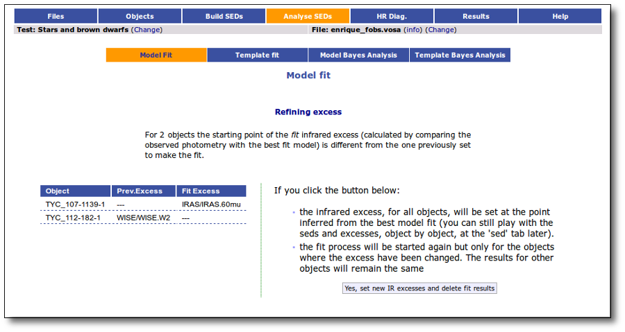
Excess fit refinement
When the fit has been done, VOSA compares the observed SED with the best fit model synthetic photometry and makes a try to redefine the start of infrared excess as the point where the observed photometry starts being clearly above the model. See the Excess help for more details.
If for some objects the IR excess starting point calculated in this way is different from the one previosly calculated by the automatic algorithm, VOSA offers you the option to "Refine excess". If you click the corresponding button you will see the list of objects where this happens, the filters where excess starts according to both algorithms for each case, and the possibility of marking the start of infrared excess in the point flagged by the fit refinement instead of the one previously calculated by VOSA. If you choose to do this, and given that this would change the number of points actually used in the fit for those objects, the fit results are deleted for these objects and the fit process is restarted for them (the results for other objects will remain unchanged). But, in what follows, the IR starting point will be the one suggested by the previous fit.
Synthetic photometry
Each theoretical spectra is a function Fi(λ) with units erg/cm2/s/Â.
Each filter is represented by a dimensionless response curve Gf(λ)
The synthetic photometry corresponding to the Fi spectra when it is observed through the filter Gf can be expressed as an integral:
$$F_{i,f}=\int_{\lambda}F_i(\lambda) \ N_f(\lambda) \ d\lambda$$
where Nf(λ) is the normalized filter response function defined as:
$$N_f(\lambda) = \frac{G_f(\lambda)}{\int G_f(x) \ dx}$$
Total flux and Bolometric luminosity
The best fitting model is used to infer the total observed flux for each source of the sample.
We note that if the model reproduces the data correctly, this correction is much more accurate
than the one obtained using a bolometric correction derived only from a color.
Total observed flux
The total theoretical flux for the object would be calculated as the integral of the whole model (multiplied by the corresponding Md factor):
$$F_M = \int {\rm Md \cdot F_M}(\lambda) \ d\lambda$$
In order to estimate the total observed flux for the object, we want to substitute the fluxes
corresponding to the observing filters by the observed ones, so that as much as the flux as
possible comes from the observations.
$${\rm Ftot} = \int{\rm Md \cdot F_M(\lambda) \ d\lambda} \ + {\rm Fobs} - {\rm Fmod} $$
The theoretical density flux corresponding to the observed one $\rm F_{o,f}$ can be calculated using the normalized filter transmision $N_f$:
$$F_{M,f} = \int {\rm Md \cdot F_M}(\lambda) \cdot N_f(\lambda) \ d\lambda$$
In order to calculate the total observed flux, we have to estimate de amount of overlaping among diferent observations. In order to do that we, first, approximate the coverage of each filter using its effective width, then we identify spectral regions where there is a continues filter coverage an, for each of those regions, we define a "overlapping factor" as:
$$ {\rm over}_r = \frac{\sum {\rm W}_i}{\rm (\lambda_{max,r} - \lambda_{min,r})}$$
using these overlapping factors we can estimate the degree of oversampling in each region by the fact that several observations are sampling the same range of the spectra. And we can approximate the total observed flux as:
$$ {\rm Fobs} = \sum_f\frac{ {\rm F}_{o,f} \cdot {\rm W}_{eff,f}}{ {\rm Over_f}} $$
And the same for the corresponding contributions from the model:
$$ {\rm Fmod} = \sum_f\frac{ {\rm F}_{M,f} \cdot {\rm W}_{eff,f}}{ {\rm Over_f}} $$
Thus, the total flux is given by:
$${\rm F}_{\rm tot} = F_M + \sum_f\frac{ [ {\rm F}_{o,f} - {\rm F}_{M,f}] \cdot {\rm W}_{eff,f}}{ {\rm Over_f}} $$
where $F_{M,f}$ and $F_{o,f}$ are the model and observed flux densities corresponding to the filter $f$.
The corresponding error in the total flux is calculated as:
$$ \Delta {\rm Fobs} = \sqrt{ \sum_f \left(\frac{ \Delta{\rm F}_{o,f} \cdot {\rm W}_{eff,f}}{ {\rm Over_f}}\right)^2 } $$
You can see a
detailed example about this calculations.
Bolometric luminosity
The tool scales the total observed flux to the distance provided by the user
and therefore estimates the bolometric luminosities of the sources in the sample
(in those cases where the user has not provided a realistic value of the distance,
a generic value of 10 parsecs is assumed):
$$L(L_{\odot}) = 4\pi D^2 F_{obs}$$
$$\left(\frac{\Delta L}{L}\right)^2 = \left(\frac{\Delta F_{obs}}{F_{obs}}\right)^2 + 4 \left(\frac{\Delta D}{D}\right)^2 $$
Estimate of parameter uncertainties
VOSA uses a grid of models to compare the observed photometry with the theoretical one. That means that only those values for the parameters (Teff, logg, metallicity...) that are already computed in the grid can be the result of the fit. For instance, if the grid is calculated for Teff=1000,2000,3000 K, the best fit temperature can be 2000K, but never 2250K (because there is not a 2250K model in the grid to be compared with the observations). But this only means that the model with 2000K, reproduces the observed SED better that the other models in the grid. And it could happen that, if it were in the grid, the model with 2200K were a better fit.
Thus, by default, VOSA estimates the error in the parameters as half the grid step, around the best fit value, for each parameter. For instance, if we obtain a best fit temperature Teff=3750K for the Kurucz model, and given that the Kurucz grid is calculated at 3500,3750,4000...K, the grid step around 3750 is 250K and the estimated error in Teff will be 125K.
Statistical approach
In order to obtain parameter uncertainties with a more statistical meaning, VOSA offers the option to "Estimate fit parameter uncertainties using an estatistical approach". If you mark this option the fit process will be different.
Taking the observed SED as the starting point, VOSA generates 100 virtual SEDs introducing a gaussian random noise for each point (proportional to the observational error). In the case that a point is marked as "upper limit" a random flux will be generated between 0 and ${\rm F}_{uplim}$ following a uniform random distribution.
VOSA obtains the best fit for the 100 virtual SEDs with noise and makes the
statistics for the distribution of the obtained values for each parameter. The standard deviation for this distribution will be reported as the uncertainty for the parameter if its value is larger that half the grid step for this parameter. Otherwise, half the grid step will be reported as the uncertainty.
Although this means making 101 fit calculations for each object (instead of only one) the process time is not multiplied by 101. It takes only a little longer (around twice).
Estimate of stellar radius and mass
We can use the value of Md and the distance $D$ to estimate the stellar radius:
$$M_d = \left(\frac{R}{D}\right)^2 $$
$$R_1 \equiv \sqrt{D^2 M_d} $$
$$\Delta R_1 = R_1 \frac{Δ D}{D} $$
But we can estimate the radius also using $T_{eff}$ and $L_{bol}$.
$$L_{bol} = 4\pi\sigma_{SB} R^2 T_{eff}^4$$
$$R_2 = \sqrt{L_{bol}/(4\pi\sigma_{SB} T_{eff}^4)}$$
$$\Delta R_2 = R_2 \sqrt{\frac{1}{4} \left(\frac{\Delta L_{bol}}{L_{bol}}\right)^2 + 4 \left(\frac{\Delta T_{eff}}{T_{eff}}\right)^2}$$
We can estimate also the mass using $logg$ and $R$
$$ g = \frac{G_{Nw}M}{R^2} $$
$$ M = 10^{logg} R^2 / G_{Nw} $$
In this formula we can use either $R_1$ or $R_2$ to obtain two different estimate of the mass:
$$ M_1 = 10^{logg} R_1^2 / G_{Nw} $$
$$\Delta M_1 = M_1 \sqrt{\ln(10)^2 (\Delta logg)^2 + 4 \left(\frac{\Delta R_1}{R_1}\right)^2} $$
$$ M_2 = 10^{logg} R_2^2 / G_{Nw} $$
$$\Delta M_2 = M_2 \sqrt{\ln(10)^2 (\Delta logg)^2 + 4 \left(\frac{\Delta R_2}{R_2}\right)^2} $$
WARNINGS.
Take into account that the values obtained, both for the mass and radius, will be make sense only if the value for the Distance is realistic. What's more, these values will be more trustable when Fobs/Ftot is closer to 1. Otherwise, the obtained values could not be realistic.
In the other hand, given that the uncertainty of $logg$ given by models is typically large, and SED analysis is not very sensible to the value of logg, take into account that the value of the Mass obtained using logg could be far from real.
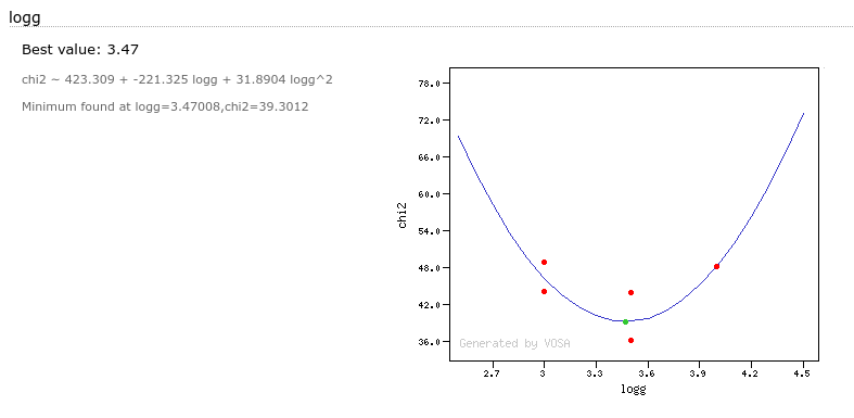
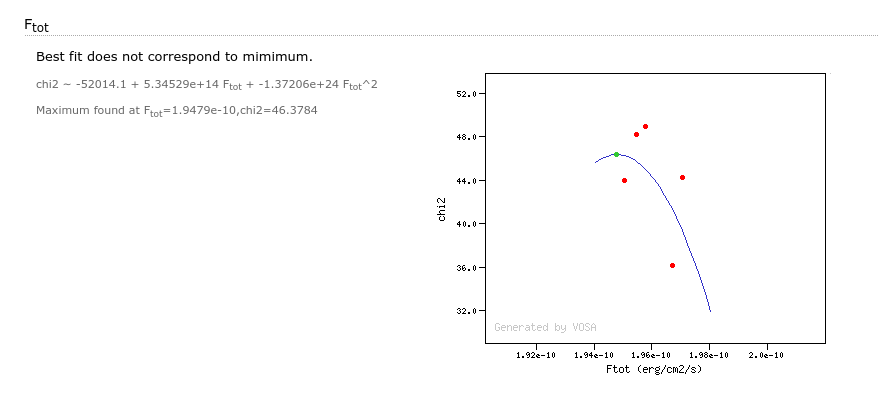
Parameter polynomial fit
When you go to see all the fits for a particular object you will also see a section named "Parameter polynomial fit".
For each fit parameter, VOSA will take into account all the values obtained in the best fits and try to adjust a 2 degree polynomial to the (param,chi2) points.
If this polynomial has a minimum and this minimum is in the range between the minimum and maximum values obtained for this parameter, VOSA will offer this value as possible "best fit value" for this parameter, trying to go further than the constraints due to the discrete nature of the model grid.
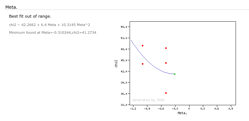
In some cases a mimimum is found but this is out of the range given by the obtained parameter values in the fit. In this case VOSA does not recommend the use of this value.
It can also happen that the parabola fit does not have a minimim but a maximum. Of course, the value of the parameter at the maximum does not provide better information.
Partial refit
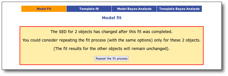
After you have finished the fit process, sometimes it is useful to make small changes in the SED for some objects and repeat the fit. But, when your file contains many objects it is boring and slow to repeat the fit process for all the objects when only a few SEDs have changed.
VOSA keeps track of what SEDs have been changed in a significant way after the fit, so that the current fit results could be not valid for those objects anymore (for instance, you edit the SED, add/remove some point, search for VO photometry, add VO photometry, change where the excess starts, change the value of extinction, etc.)
When you go back to the chi2 fit tab, VOSA will show you a message saying the the SED for some objects has been changed after the fit was finished and offers you the option of repeating the fit only for those objects. If you click in the "Repeat the fit process" button, the fit process will be done again with the same previous options (model choice, parameter ranges choices, etc) but only for the objects that have changed. The fit results for the other objects will remain the same.
A particular case is the one when you choose to refine the excess setting the start of the IR excess at the point suggested by the model fit. When you do this, the fit is repeated only for the objects where the excess have changed (the results for other objects will remain unchanged).
Example
When we access the Chi-2: Model Fit tab we see a form with the available theoretical models, so that we can choose what ones we want to use in the fit. In this case we decide to try Kurucz and BT-Settl-CIFIST models. Thus, we mark them and click in the "Next: Select model params" button.
For each of the models, we see a form with the parameters for each model and the available range of values for each of them. We choose the ranges that best fit our case and then click the "Next: Make the fit" button.
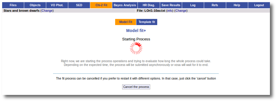
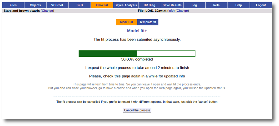
The fit process is performed asynchronously so that you don't need to stay in front of the computer waiting for the results. You can close your browser and come back later. If the fit is not finished, VOSA will give you some estimate of the status of the operation and the remaining time.
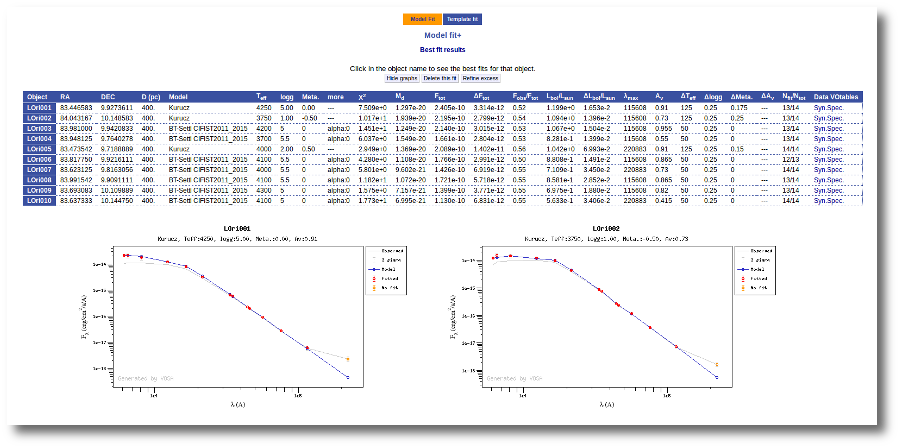
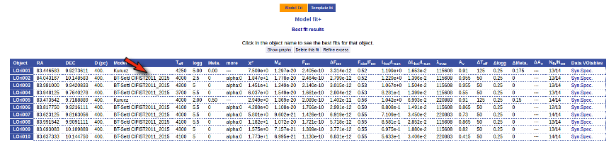
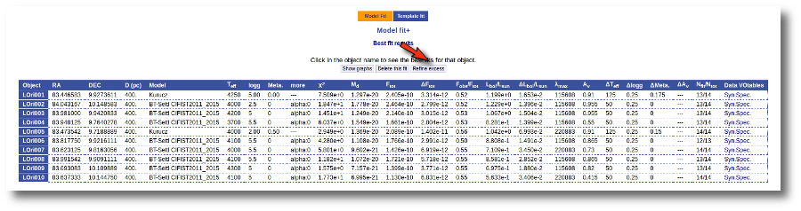
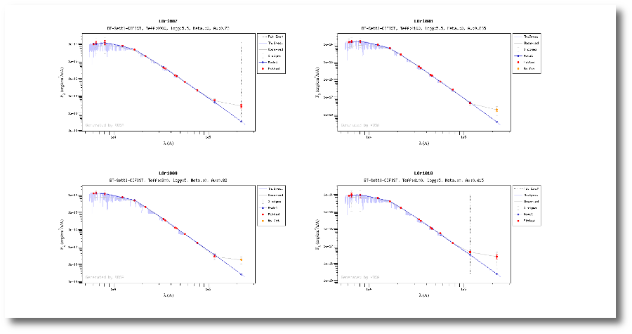
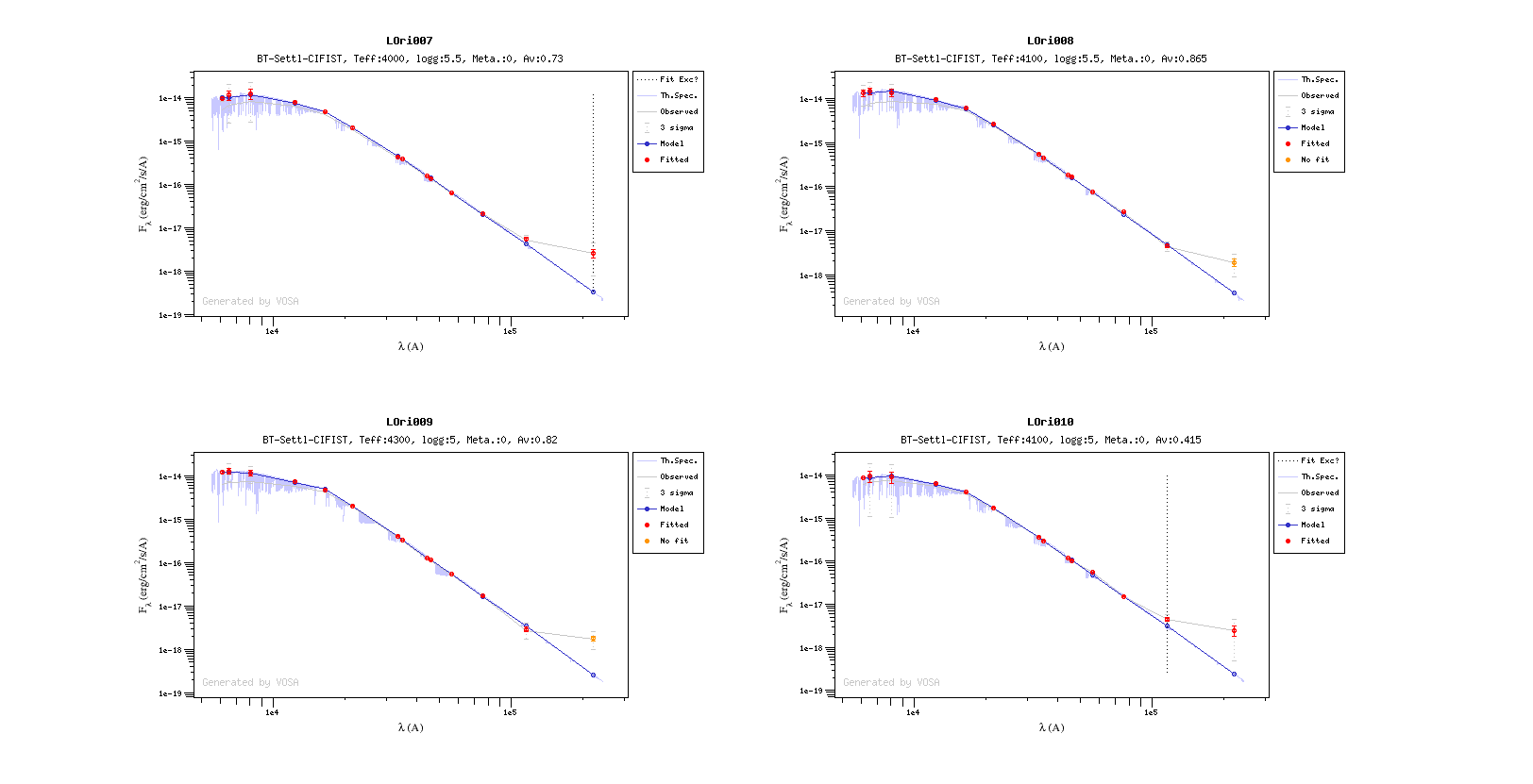
When the process finishes VOSA shows a list with the best fit model (that is, the one with a smaller value for the reduced chi-2) for each object. Optionally you can also see the best fit plots, with the observed SED and the corresponding synthetic photometry for the best fit model.
If we click in the LOri002 object name in the table we can see the 5 best fits for each collection of models. And clicking on the "See" link on the right of each fit, we can see the details about it.
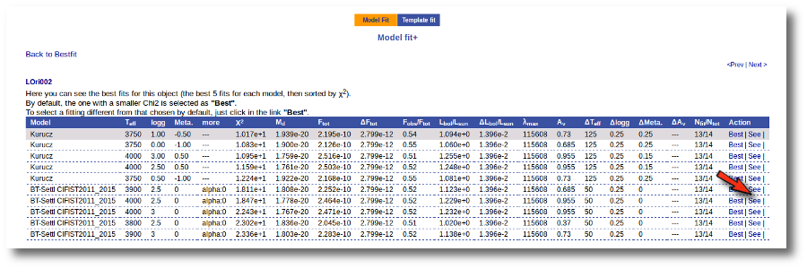
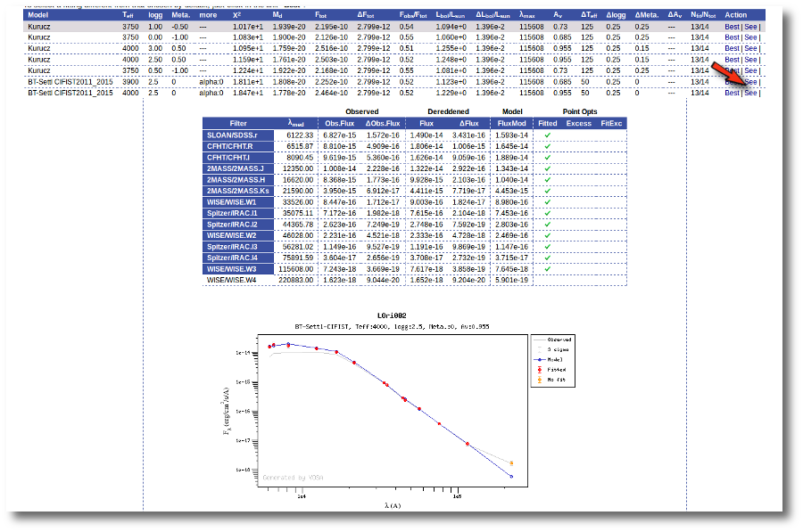
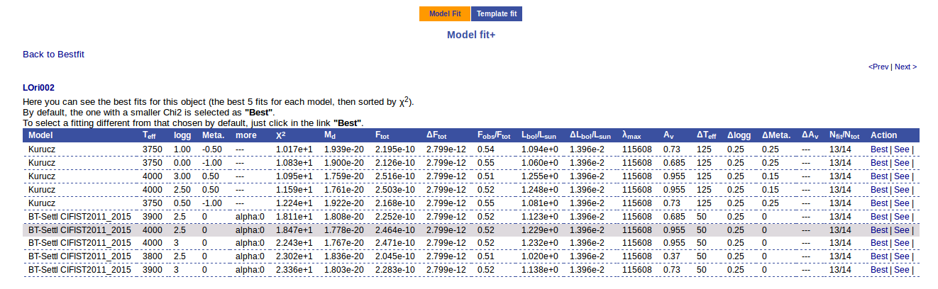
Sometimes the fit with the best Χ2 is not the one that the user considers the best one, maybe for physical reasons, taking into account the obtained values of the parameters, or maybe because one prefers a model that fits better some of the points even having a larger Χ2... Whatever the reason, we have the option to mark as Best the model that we prefer. In order to do that we just click in the Best link at the right of the fit that we prefer. In this case, just as an example, we choose the second BT-Settl one for LOri002.
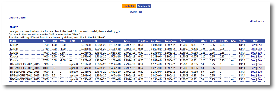
And, when we go back to the best fit list, we see that the one for LOri002 has changed.
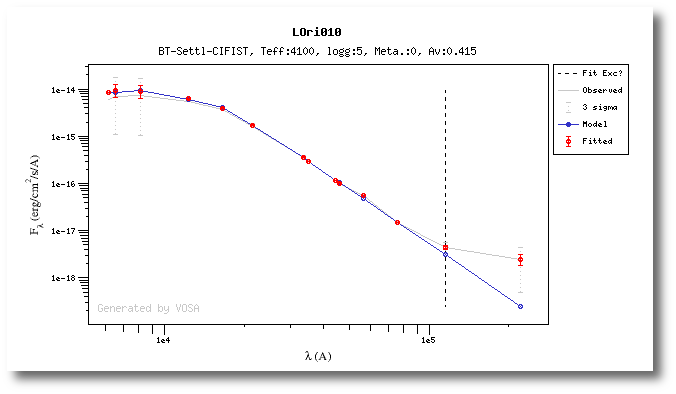
For some objects, for instance LOri10, we see a vertical dashed line in the plot at the point where the observed fluxes start being clearly above the model ones. VOSA marks it this way so that you are aware that infrared excess could start here.
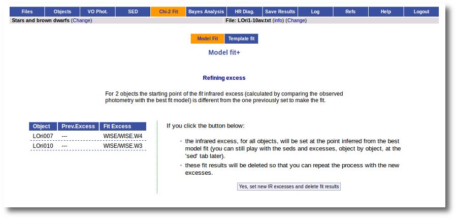
If we click in the "Refine excess" button, we can see the list of objects where VOSA detects a possible infrared excess starting at a point different from the one previously detected.
If we click the "Yes, set new IR excesses and delete fit results" button, the start of infrared excess will be flagged at the point coming from the fit comparison and these fit results will be deleted. Then we could restart the fit taking into account the new infrared excesses.
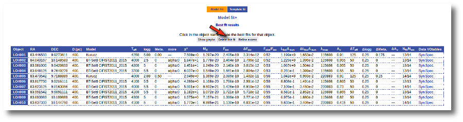
We also have the option of deleting these fit results so that we can restart the process with different options. And we do so clicking in the "Delete" button.
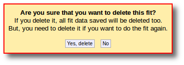
VOSA asks us for confirmation, we confirm the decision, and we see the initial form again.
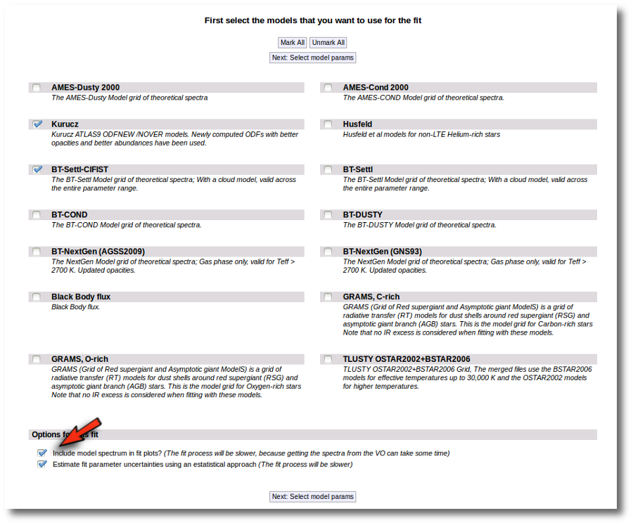
We select the same models again but we also mark the two extra options at the bottom.
When the fit process ends, we see two main differences in the results:
- The values of the estimated errors for the parameters are now different:
- The model spectrum is included in the fit plots.
| 


 Excess