Use Case: From SED fitting to Age estimation. The case of Collinder 69

[Introduction] [User data] [Upload file] [Model fit] [HR diagram] [Save Results]

Model fit.

The determination of physical parameters of astronomical objects from observational data is frequently linked with the use of theoretical models as templates.

The use, in the traditional way, of this methodology can easily become tedious and even unfeasible when applied to large amount of data. VOSA uses VO methodologies to authomatically fit several collection of theoretical models to the observed photometry for different objects

When we access the Model Fit tab we must click in the Fit link.

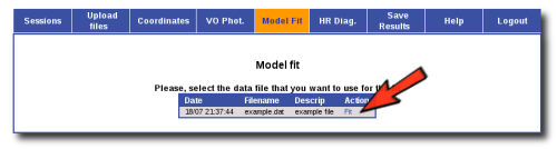
(click on the image to see full size)

Then, a list of the available theoretical models is shown, so that we can choose which of them we want to use in the fit. In this case we decide to try all the models. Thus, we mark all of them and click in the Continue button.

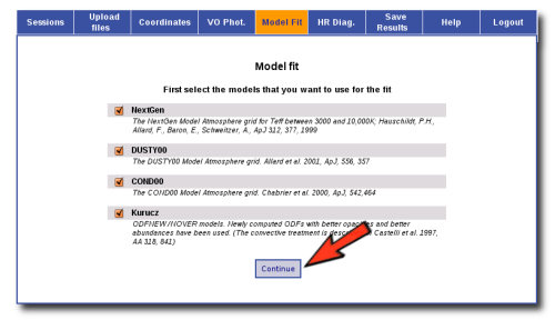
(click on the image to see full size)

For each of the models, we see a form with the parameters for each model and the available range of values for each of them. We choose the ranges that best fit our case and then click the Continue button again.

(click on the image to see full size)

The fitting process usually takes a while but in this case, with only two objects, it takes only a few seconds.

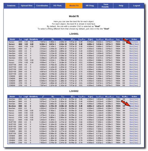
When the process finishes the tool shows us a list with the best five models for each collection, all ordered by the Χ² of the fit.

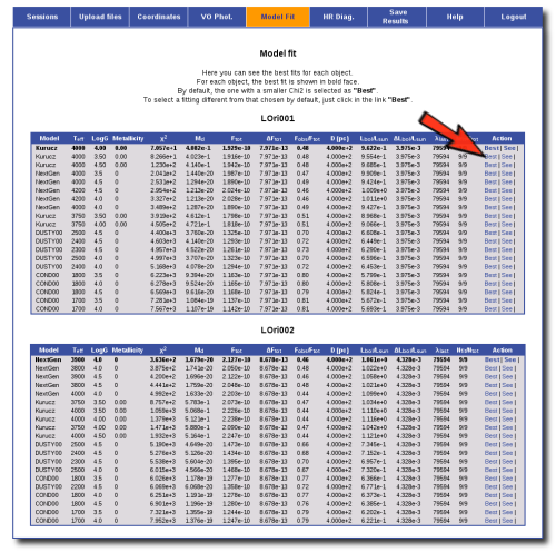
(click on the image to see full size)

In this step, we have the option of seeing a graph for each of the fits by clicking on the See link.

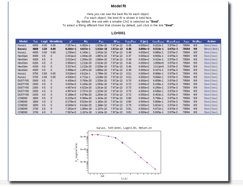
(click on the image to see full size)

Sometimes the fit with the best Χ² is not the one that the user considers the best one, maybe for physical reasons, taking into account the obtained values of the parameters, or maybe because one prefers a model that fits better some of the points even having a larger Χ²... Whatever the reason, we have the option to mark as Best the model that we prefer. In order to do that we just click in the Best link at the right of the model that we prefer. In this case we choose the second one for LOri001 and the fourth one for LOri004.

(click on the image to see full size)

The next time that we click in the Model Fit tab we have three options. We can go back to the page with the fit results, we can delete all the results so that we can start the fitting process again, and we can also see a table with the best fit results.

(click on the image to see full size)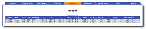

(click on the image to see full size)

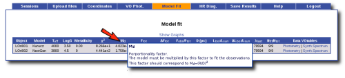
You can move your mouse over each of the table headers and a window will appear with short explanation of the concept represented in that column.

(click on the image to see full size)

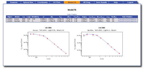
We can also see the fit graphs for all the objects clicking in the Best Graphs link.

(click on the image to see full size)

In this process we have been able to estimate some physical parameters for our objects. The models have given us the effective temperature and the surface gravity (it would have given us the metallicity too but we have fixed it to zero). Also, the total flux of the objects can be estimated using the model for those areas of the spectrum not covered by the observed photometry. And finally, using the distance given by user, the application estimates the bolometric luminosity of the object.

Object Teff Log(G) Ftot Lbol/Lsun LOri001 4000 3.5 1.916e-10 0.955 LOri002 3800 4.5 2.048e-10 1.021