Model Fit
[Introduction] [Fit] [Best Fit] [Reduced chi-square] [Excess] [Synthetic photometry] [Bolometric Luminosity]
Introduction
The main section of this application is the Model fit.
When the user clicks in the Model fit tab, a list of the files is shown. For each of them, a list of actions can be chosen:
- Fit. If the fit hasn't been done yet for this data file, this option starts the fit (and it is the only option that can be chosen). Otherwise, it shows the list of all the best fit results so that the user can choose the best one for each object (sometimes, there are reasons why the best physical fit is not the one with a smaller Χ2r and the user has the option to choose a different one as the best for a particular object).
- Best Fit. It only appears if the fit is finished. Here the user can see a table with the best fit for each object and, as an option, all the graphs for the best fits.
- Del Fit. If the user wants to start the fit process again (maybe with a different election of models or different ranges of parameters for some of them), it is necessary to delete the previous results first.
Fit
When a fitting process is started the user can choose among a list of theoretical spectra models available in the VO. Only those that are checked will be used for the fit.
In the next step the application uses the TSAP protocol (SSAP for theoretical spectra) for asking the model servers which parameters are available to perform a search. According to that, a form is built for each model so that the user can choose the ranges of parameters that he wants to use for the fit. Take into account that:
- The fitting process implies queries to VO services, data sent through the network, a lot of calculations (some done by the services themselves and some done by the application)... That means that it could take a long time to get the final results (seconds for only an object or half an hour for around 100 depending also on the load of the services).
- Using more models and wider ranges of parameters will imply a longer time for the fitting (specially if your file contains many objects) so be ready for a long waiting time in the next step.
- In some cases, the whole ranger of parameters offered by the models are not right for your objects. For instance, if you know, for whatever physical reasons, that your objects have small temperatures, choose only small temperatures in the forms to optimize the process.
- The response time has roughly linear dependence on the number of objects in the file (twice number of objects means twice waiting time). Thus, you could prefer splitting your input file in different ones (according to physical properties, pertenence to a group or simmilar reasons) better than doing all the work in an only data file.
Once the fit has been finished, the user can see a list of results for each object. The list contains the five better fits for each model and are ordered so that the smaller Χr2 are shown first.
The user can see also a simple plot for each result (with the "See" button) or can use the "Best" button to mark a different result as the preferred best one. If he does, this fit will be shown in bold face and it will be the one that will be shown in the "Best fit" table later.
Best Fit
Once a fit has been done, the user has the option to access a Best Fit with the best fit properties for each object.
A number of results are shown for each object:
- Object name, as given by the user.
- Model name that best fits the data.
- Teff: effective temperature, in K, for the model that best fits the data.
- Log(G): logarith of the gravity for the model that best fits the data.
- Metallicity: metallicity for the model that best fits the data.
- Χr2: value of the reduced chi-squared parameter for the fit (see below).
- Md: dilution factor. Value by which the model has to be multiplied to fit the data (see below).
- Ftot: Total flux (see below).
- Fobs/Ftot: fraction of the total flux obtained from the observed photometry (See below).
- D(pc): distance in pc as given by the user (if the user does not provide a value, a typical value of 10pc is used and the corresponding results are shown in italic).
- Lbol/Lsun: Bolometric luminosity (See below).
- λlast: value of the last wavelength considered for the fitting In order to avoid data with excess) (See below).
- Nfit/Ntot: Number of points coinsidered in the fitting (avoiding excess) divided by the total number of observed points (See below).
- Link to a VOtable with the observed photometry.
- Link to a VOtable with the synthetic photometry corresponding to the best fit.
- Link to a VOtable with the synthetic spectra corresponding to the best fit.
Reduced chi-square
The fit process minimizes the value of Χr2 defined as:

Where:
| N: |
Number of photometric points. |
| np: |
Number of fitted parameters for the model.
(N-np are the degrees of freedom associated to the chi-square test) |
| Yo: |
observed flux. |
| σo: |
observational error in the flux. |
| Ym: |
theoretical flux predicted by the model. |
| Md: |
Multiplicative dilution factor, defined as:

being R the object radius and D the distance between the object and the observer.
It is calculated as a result of the fit too. |
Excess
During the fitting process, the tool detects possible infrared excesses.
Since the theoretical spectra correspond to stellar atmospheres, for the calculation of the Χr2 the tool only considers those data points of the SED corresponding to bluer wavelengths than the one where the excess has been flagged.
The excesses are detected by calculating iteratively in the mid-infrared (adding a new data point from the SED at a time) the α parameter from Lada et al. (2006) (which becomes larger than -2.56 when the source present an infrared excess).
The last wavelength considered in the fitting process and the ratio between the total number of points belonging to the SED and those really used are displayed in the results tables.
Synthetic photometry
Each theoretical spectra is a function Fi(λ) with units erg/cm2/s/Â.
Each filter is represented by a dimensionless response curve Gf(λ)
The synthetic photometry corresponding to the Fi spectra when it is observed through the filter Gf can be expressed as an integral:

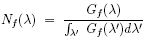
where Nf(λ) is the normalized filter response function defined as:
The numerical integrals are calculated using a 5-point Newton-Cotes formula (Boole's rule) which is given by:

In order to be able to apply this numerical method it is mandatory that increment in the x axis (h) is constant through the integration interval, and that the number of intervals is a multiple of four. Thus, before doing the integral, both the filter response and the synthetic spectra are resampled, if necessary (without loosing resolution), to accomplish the requirements.
Total flux and Bolometric luminosity
The best fitting model is used to infer the total observed flux for each source of the sample. We note that if the model reproduces the data correctly, this correction is much more accurate than the one obtained using a bolometric correction derived only from a colour.
Total observed flux
The total theoretical flux for the object would be calculated as the integral of the whole model (already multiplied by the corresponding Md factor):
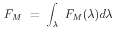
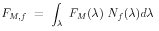
In order to estimate the total observed flux for the object, we want to substitute the fluxes corresponding to the observing filters by the observed ones, so that as much as the flux as possible comes from the observations. The total theoretical flux for a filter Gf is given by:
The total flux observed through the filter Gf is given by:

where FGf is the observed flux density. Thus, the total observed flux is given by:

This takes into the account the model to correct from possible intersections among the filters wavelength coverage.
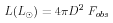
Bolometric luminosity
The tool scales the total observed flux to the distance provided by the user and therefore estimates the bolometric luminosities of the sources in the sample (in those cases where the user has not provided a realistic value of the distance, a generic value of 10 parsecs is assumed):
|