Binary Fit
The idea of "binary fit" appears when we face the case where an observed SED cannot be fitted well with a single theoretical model (that is, the flux comming from a single object) but it seems that it could be fitted well adding a second model (the flux comming from a second object).
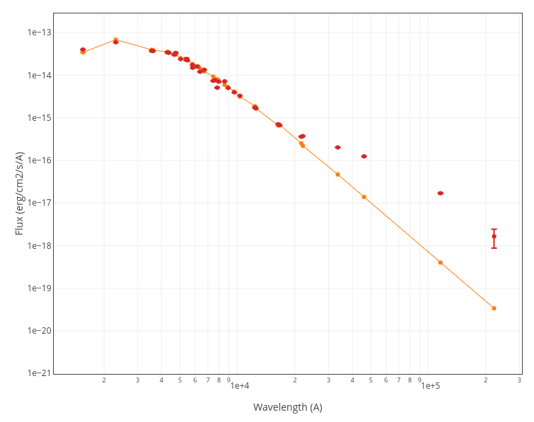
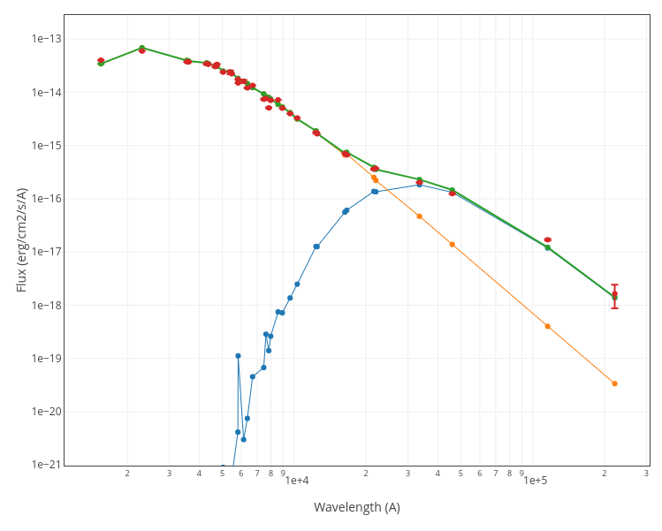
A typical case could be a SED with a clear infrared excess where we could have two clear contributions: the flux from a somewhat hotter object for the main part of the SED (in orange in the plot), and the flux coming from a colder object (cold star, dust...) for the infrared excess (in blue in the plot).
Binary Fit procedure
We can write this down as the fact that we want to represent the observed flux as the linear combination of two different models (the fluxes coming from two different objects), that is:
$$ {\rm F}_{\rm obs}(x) \sim A \ {\rm F}_{\rm a}(x) + B \ {\rm F}_{\rm b}(x) $$
We know the observed fluxes ${\rm F}_{\rm obs}(x)$, and we know what theoretical grids to use for objects a and b (these are inputs from the user). We need to find the best parameters for each theoretical model and both dilution factors $A$ and $B$.
The method to do this, and estimate model parameters and A and B, is trying to minimize $\chi^2$ defined as:
$$\chi^2 = \sum_x \left(\frac{A \ {\rm F}_{\rm a}(x) + B \ {\rm F}_{\rm b}(x) - {\rm F}_{\rm obs}(x)}{\Delta{\rm F}_{\rm obs}(x)}\right)^2 $$
Most of the explanations given in the chi-square model fit section are also valid for the binary fit. But there are very important differences.
We will focus here mostly in those aspects that are specific of the binary fit.
In the case of the one model chi-square typical fit, VOSA compares the observed SED with the synthetic photometry of all the models in the grid, calculates the best $M_d$ for each case and chooses the model so that chi-square is minimal. And this process, trying all the posible model parameter space, is quite deterministic as $M_d$ is calculated for each case, not estimated, fitted, etc, but calculated as one of the fit results.
But this is imposible for the binary fit. Here we can calculate one of the two dilution factors ($A$ or $B$) but we need to estimate the other one in a different way. And there is no deterministic way in which we can calculate all the parameters. For instance, if we rewrite our equation above as:
$$ {\rm F}_{\rm obs}(x) \sim A \ \left( \ {\rm F}_{\rm a}(x) + R_{\rm f} \ {\rm F}_{\rm b}(x) \ \right) $$
we can make a loop through all the models (a and b) parameter space, try/estimate a value of $R_{\rm f}$, and then calculate the corresponding value for $A$. And we will have the best fit for that "estimation".
but we will never be sure that we have chosen the best posible value for $R_{\rm f}$.
In most of the cases, the success of the binary fit process relies in a good estimation of $R_{\rm f}$ (then, a loop of values around that estimation could help to refine the results).
We are going to explain briefly the algorithm used by VOSA to estimate the best binary fit parameters.
VOSA Binary Fit algorithm
There are several posible ways to implement this process. After many tests we have chosen the one explained here as a compromise of the time and resources used by the process and the accuracy of the results. You can get an analysis of the quality of the results obtained at the Binary Fit Quality
section. And, please, remember not to use the binary fit as a black box that you can use and trust with your eyes closed.
Remember that the main equation can be writen as:
$$ {\rm F}_{\rm obs}(x) \sim A \ \left( \ {\rm F}_{\rm a}(x) + R_{\rm f} \ {\rm F}_{\rm b}(x) \ \right) $$
1.- Loop in models parameters space.
we try all the posible parameter values for both models (a and b). For instance, just to simplify the notation, we can imagine that the only parameter for these grids is the temperature and, thus, we try all the posible pairs (Teff$_{\rm a}$, Teff$_{\rm b}$).
For each of these pairs we need to estimate a value of $R_{\rm f}$ (and $A$) that we think that will make sense.
To do this first estimation we need two equations to obtain values for A and B (or, actually, A and $R_{\rm f}$).
To get these two equations we take two different sets of points in the observed SED. For instance, one of them starting at short wavelengths and the other, on the contrary, starting at the longest wavelengths.
There are different approaches that we could use here, depending of the size of the sets and other conditions. But we have chosen one of the simplest ones:
- Use the equation above (the full linear combinaton of both models) and require that it fits well both the first and last points of the observed SED. That is, we use a set size = 1 for both SED ends.
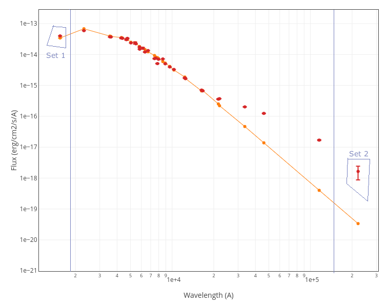
We can thus apply the corresponding equations and, for each point in the model parameter space, we get a first estimation of ($A$ and $R_{\rm f}$) as the values that fit well sets 1 and 2.
(teff$_{\rm a}$, teff$_{\rm b}$...)$_i$ $\Rightarrow$ (A,$R_{\rm f,estim}$)$_i$
(teff$_{\rm a}$, teff$_{\rm b}$...)$_j$ $\Rightarrow$ (A,$R_{\rm f,estim}$)$_j$
...
1.- Loop around first estimation.
After the first estimations, for each point in the model parameter space (teff$_{\rm a}$, teff$_{\rm b}$...)$_i$ , we define an interval of possible values of $R_{\rm f}$ ($R_{\rm f,min}$...$R_{\rm f,estim}$...$R_{\rm f,max}$) around this first estimate and we check if the global value of $\chi^2$ (using the full combination of models over the complete observed SED) improves when making a loop around the first estimation. In this way, for each pair of models we obtain a series of:
(teff$_{\rm a}$, teff$_{\rm b}$...)$_i$ $\Rightarrow$ (A,$R_{\rm f,best}$)$_i$ $\Rightarrow$ $\chi^2_i$
(teff$_{\rm a}$, teff$_{\rm b}$...)$_j$ $\Rightarrow$ (A,$R_{\rm f,best}$)$_j$ $\Rightarrow$ $\chi^2_j$
...
And we finally select the one that gives the smallest value of $\chi^2$. And the corresponding values for model parameters, A and $R_{\rm f}$ that lead to this best fit.
(teff$_{\rm a}$, teff$_{\rm b}$...)$_{Best}$ $\Rightarrow$ (A,$R_{\rm f,Best}$)$_i$ $\Rightarrow$ $\chi^2_{Best}$
These are the values that will be returned by the binary fit process.
| 
 Templates Bayes