Version 7.5, July 2022
Table of contents
Introduction
VOSA (VO Sed Analyzer) is a tool designed to perform the following tasks in an automatic manner:
- Read user photometry-tables.
- Query several photometrical catalogs accessible through VO services (increases the wavelength coverage of the data to be analyzed).
- Query VO-compliant theoretical models (spectra) and calculate their synthetic photometry.
- Perform a statistical test to determine which model reproduces best the observed data (optionally fitting at the same time the optimal interstellar extinction).
- Provide the likelihood of the model parameters (and the interestellar extinction).
- Use the best-fit model as the source of a bolometric correction.
- Provide the estimated bolometric luminosity for each source.
- Generate a Hertzsprung-Russel diagram with the estimated parameters.
- Provide an estimation of the mass and age of each source.
See this documentation in a single page.
This can be useful to print or to search text, but take into account that it is a large page and can be heavy to load for your browser.
Input files
There are two main ways to start working with VOSA:
- Uploading a VOSA-format input file with your data (or selecting a previously uploaded one).
VOSA is mainly designed to work with several objects at the same time so that the same or equivalent operations are performed on all the objects. The information about these objects (and optionally, user photometry data for them) must be uploaded by the user in an input ascii file with an special format.
Please, read carefully how to write an input file in VOSA-format.
- Making a simple search for a single object giving its coordinates.
Using these coordinates VOSA builds an input file and uploads it automatically to the application.
And, at any time, you can select a previously uploaded file and continue with it in the same point where you left the work. Below you can see details about these three options.
Upload data files
Whenever you click on the "Files" tab, you have the option of uploading a new file.
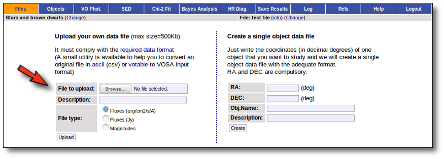
In order to do that you have to:
- Give a description for the file.
- Specify if the photometric points in your file are expressed as magnitudes or fluxes (in erg/cm2/s/A o Jy).
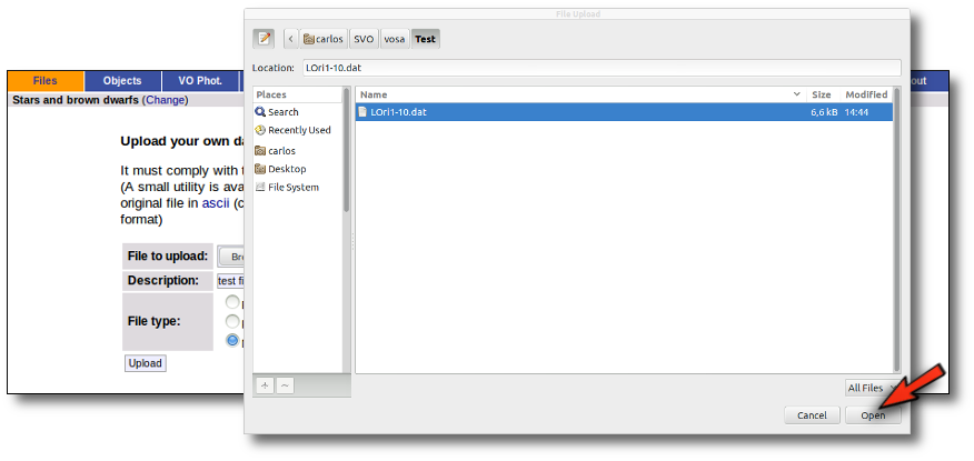
- Select a file.
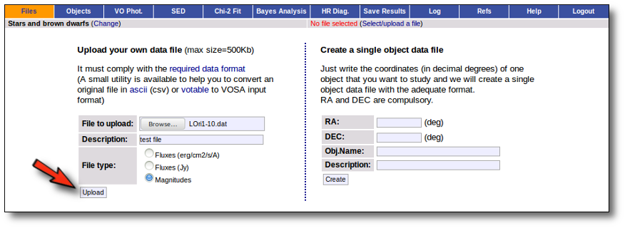
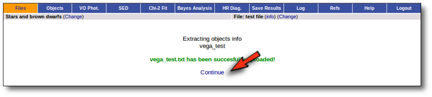
When you click the "Upload" button, your file is transfered to the VOSA server and then it starts been analyzed. This can take a while if the file is large.
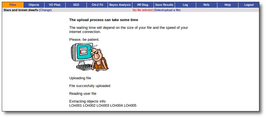
If everything is OK, you will get a message saying so. Please, click in "Continue" to go ahead.
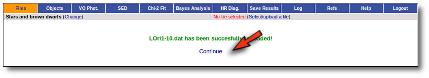
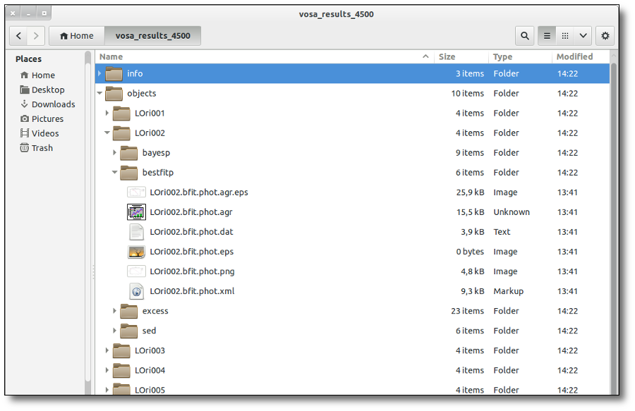
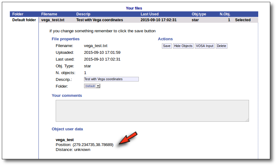
You will go back to the "Files" page. Now you can see the details about the just uploaded file, that will be already available to work with it.
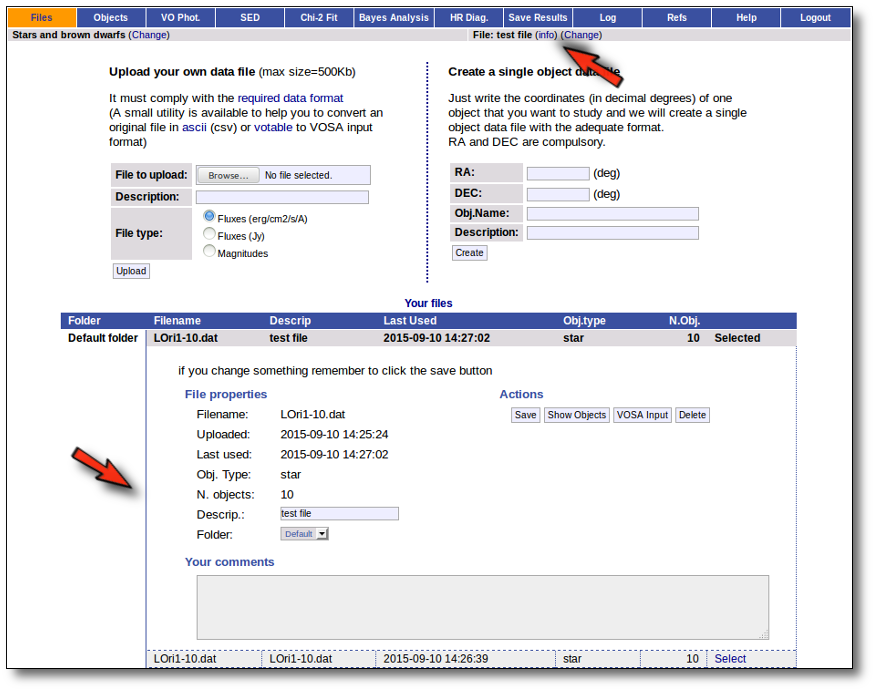
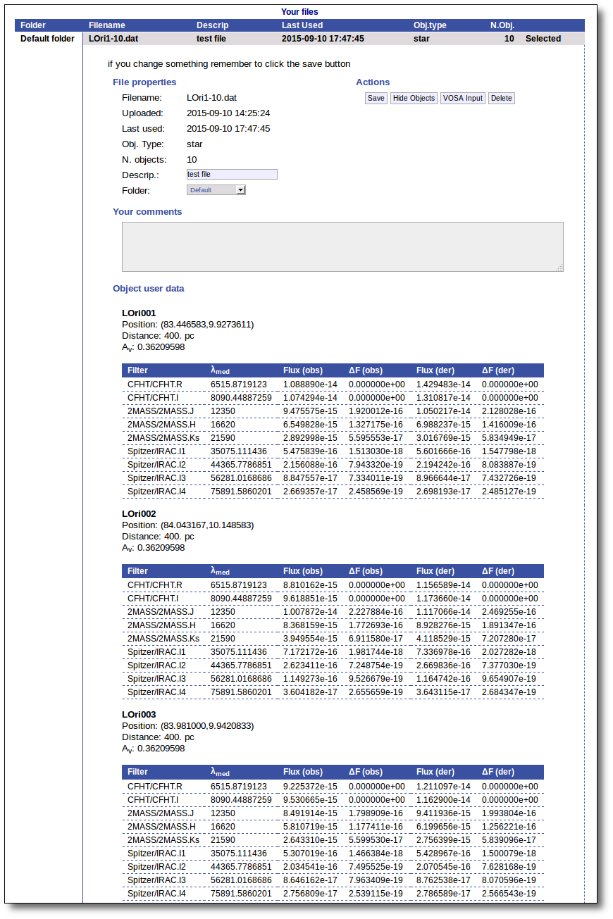
Even if there were not errors detected by VOSA, it is a very good idea to check if the format of your file has been correctly understood. So, please, whenever you upload a new file, click in the "Show Objects" button to see the information that VOSA has save for each object.
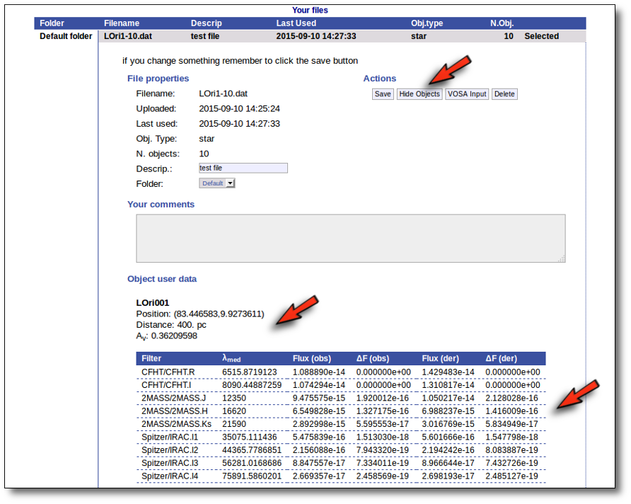
For each object in the file you should see its properties (name, position, extinction, distance...) and its photometric points. See if this is what you expected. If not, delete this file, check your input file and upload it again.
(while you are seeing the objects details, the "Show Objects" button is changed to "Hide Objects": you can use this one to hide the details)
Once the file is uploaded and you have checked that everything is ok, you can go to any of the other tabs in the index above and start working.
VOSA file format
VOSA is mainly designed to work with several objects at the same time so that the same or equivalent operations are performed on all the objects. In order to do this, we have defined a format so that the user can upload the info about these objects together with user photometric data.
Thus, the main way to use vosa is to upload a VOSA input file with this format (or selecting a previously uploaded one).
Nevertheless, we have added the Single Object Search so that you can directly search for a single object using its coordinates. See more information below.
Required input file format
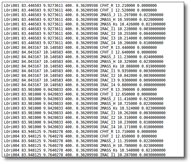
The uploaded file must be an ascii document with a line for each photometric point.
Each line should contain 10 columns:
 ----------------------------------------------------------------------------
| object  | RA  | DEC | dis | Av | filter | flux | error | pntopts | objopts |
| ---     | --- | --- | --- | ---| ---    | ---  | ---   | ---     | ---     |
| ---     | --- | --- | --- | ---| ---    | ---  | ---   | ---     | ---     |
- 1: a one word text label, without spaces or special characters, that corresponds to the object name. See (1).
- 2: the RA, in deg, corresponding to the object in J2000 equinox. See (2).
- 3: the DEC, in deg, corresponding to the object in J2000 equinox. See (2).
- 4: the distance to the object in parsec. See (4).
- 5: the AV parameter defining the extinction. See (5).
- 6: a label corresponding to the name of the filter. It must be in the list of available filters . See (6).
- 7: the flux in erg/cm2/s/A, Jy or magnitude. See (7).
- 8: the observed error in the flux (in erg/cm2/s/A) or magnitude. See (8).
- 9: options specific for this photometric point. See (9).
- 10: options specific for this object (they must be repeated in each line corresponding to the same object). See (10).
Take into account that:
- (1) The only mandatory value is the object name (you can use the real one or some label of your like). The other columns can be writen as '---' (please, don't let them blank nor write '...' instead of '---') if you don't know the right value or don't want to specify it.
- (1) Only alphanumeric characters (letters and numbers) should be used in object names. A very short list of special characters are allowed too, in particular the "_" (underscore) character. Two special "tricks" can be used if necessary:
- Asterisks are forbiden in object names. But if you include the special string "_AST_" in an object name it will be treated as ans asterisk (*) for object name resolution. For instance, if you use EM_AST_SR3 it will be submited to simbad as EM*SR3.
- If you include a "_" character in the object name (not as part of _AST), it will be treated as an space for object name resolution. This can be useful if you are using real object names that contain spaces (for instance, the variable star "R Aql") and you need to use the actual name so that it can be resolved by VOSA using VO services. In a case like that, write "R_Aql" as the object name in the file.
- (2) Coordinates (as accurate as possible) are necessary to obtain photometry from VO catalogues.
If unknown, you can write RA and DEC as '---'. In that case, if you have given the right object name in the first column, you can use the Objects:Coordinates section to find the coordinates for the object using Sesame.
- (4) The distance to the object is necessary to compute the Bolometric Luminosity.
If you don't know the distance, write it as '---' and an assumed distance of 10pc will be used in the calculations.
You can also provide a value for the error in the distance. In order to do that write D+-ΔD (for instance: 100+-20), without spaces (Remember to write both symbols, + and -, together, not a ± symbol or something else; otherwise vosa will not understand the value)
- (5) The value of visual extinction and the the extinction law by Fitzpatrick (1999), improved by Indebetouw et al (2005) in the infrared, are used to deredden the user and VO photometry in a standard way. No reddening correction is applied if Av is set to '---' or zero. Take a look to the corresponding Credits Page for more information.
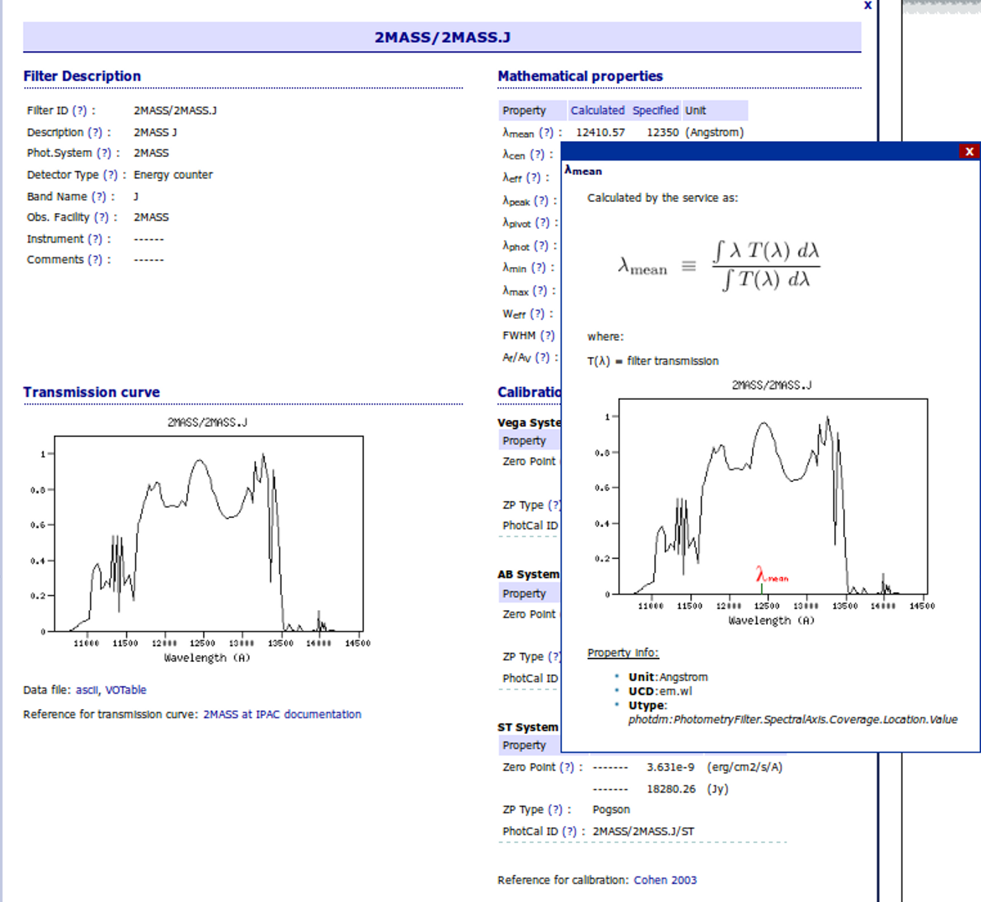
- (6) We use the SVO Filter Profile Service as the source for filter names and properties. Check it to see if the filter corresponding to your observed data is in the list (if not, contact us and we will try to include it).
- (7) If your input file containes magnitudes or fluxes in Jy, please, be careful to mark the corresponding checkbox when uploading the file. If not, we will understand the values as fluxes in erg/cm2/s/A).
- (7) If your data are given in Jy, we will transform them to erg/cm2/s/A using the λ value given by the SVO Filter Profile Service. If you prefer other λ value, please, transform the fluxes to erg/cm2/s/A before uploading your file.
- (7) If your data are given as magnitudes, we will transform them to erg/cm2/s/A using the properties (photometric system, zero point, etc) given by the SVO Filter Profile Service. If you prefer a different transformation, do it yourself and upload the file with fluxes in erg/cm2/s/A.
- (8) Errors must be specified in the same units as the fluxes (or magnitudes).
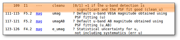
- (9) You can specify certain options for each photometric point including a special keyword in this column. By now these options are available:
- "---" : nothing special for this point.
- "nofit" : this point will be included in the SED and in all the plots. But it will NOT be used for the fit.
- "uplim" : this point will be considered an upper limit.
- "mag" : the flux and error included in columns 7 and 8 are given as magnitudes.
- "erg" : the flux and error included in columns 7 and 8 are expressed are given in erg/cm2/s/A.
- "jy" : the flux and error included in columns 7 and 8 are expressed are given in Jy.
These three last options can be mixed in the file. If "mag","erg" or "jy" is included for one point, this point will we handled accordingly even though the global "file type" that you choose to upload is different. If you don't specify one of these options for one point, the file type will be used as default.
- (10) You can specify certain options for each object including a special keyword in this column. By now these options are available:
- "---" : nothing special for this object.
- "Av:av_min/av_max" : Range of values for Av. If you give a range here, the visual extintion will be considered as an additional parameter in model fit, bayes analysis and template fit. See the corresponding section for details.
- "Veil:value" : value in Angstroms so that photometric points with smaller wavelength will be considered to present UV/blue excess.
- "excfil:FilterName" : name of the filter where infrared excess starts for this object.
In the future, other options could be implemented.
Please, check in advance that your file conforms to these requirements. Next, after uploading it, you can try to see the analyzed contents of the file in "Upload files → Show". If what you see does not correspond to what you expect it will probably mean that there is something wrong in your data file. Delete it from the system, try to correct the mistake and upload it again.
Examples of valid files
1.- A complete file
Obj1 19.5  23.2 80 1.2 DENIS/DENIS_I     5.374863e-16 4.950433e-19 ---    Av:0.5/5.5
Obj1 19.5  23.2 80 1.2 CAHA/Omega2000_Ks 2.121015e-16 1.953527e-19 ---    Av:0.5/5.5
Obj1 19.5  23.2 80 1.2 Spitzer/MIPS_M1   6.861148e-15 1.390352e-16 nofit  Av:0.5/5.5
Obj2 18.1 -13.2 80 1.2 WHT/INGRID_H      1.082924e-14 2.194453e-16 ---    ---
Obj2 18.1 -13.2 80 1.2 2MASS/2MASS_J     2.483698e-17 2.287603e-19 ---    ---
In this file we have two different objects, their positions (RA and DEC), the distance to the objects, the AV parameter and some values of the photometry (three for Obj1 and two for Obj2). For the first object, the MIPS_M1 will not be used for the fit, and Av will be considered as a fit parameters with values from 0.5 to 5.5
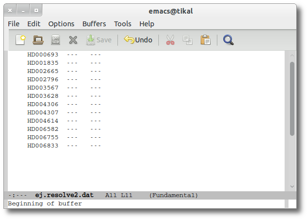
2.-Only object names
BD+292091 --- --- --- --- --- --- --- --- ---
HD000693  --- --- --- --- --- --- --- --- ---
HD001835  --- --- --- --- --- --- --- --- ---
This file is also correct, and although we have little information in it, VOSA can try to find some more data about these objects so that the analysis can be performed. Assuming that the names for the three objects are the real ones, we can try to find these objects coordinates. Then, using these coordinates, some observed photometry could be retrieved from VO catalogues, and so on.
2.-A mixed case
#objname  RA   DEC     DIS Av  Filter          Flux               Error             PntOpts ObjOpts
#=======  ===  ======= === === =============== ================== ================= ======= =======
BD+292091 ---  ---     --- --- 2MASS/2MASS_J   7.14724167946E-14  5.14601400921E-16 ---     ---
BD+292091 ---  ---     --- --- 2MASS/2MASS_H   3.69142119547E-14  2.3625095651E-16  ---     ---
Obj2      18.1 -13.2   80  1.2 DENIS/DENIS_I   1.082924e-14       2.194453e-16 	    ---     ---
Obj2      18.1 -13.2   80  1.2 2MASS/2MASS_J   2.483698e-17       2.287603e-19 	    ---     ---
HD000693  2.81 -15.467 --- --- ---             ---  		  --- 		    ---     ---
HD001835  ---  ---     --- 1.4 ---             --- 		  --- 		    ---     ---
Obj3      19.5 23.2    80  1.2 Omega2000_Ks    2.121015e-16 	  1.953527e-19 	    ---     ---
Obj3      19.5 23.2    80  1.2 Spitzer/MIPS_M1 6.861148e-15 	  1.390352e-16 	    ---     ---
HD003567  ---  ---     --- --- ---             ---           	  --- 		    ---     ---
You can combine in the same file objects with different type of information. Just keep in mind that each line must have 10 columns and, when you want to leave a data blank, you must write it as '---'.
And remember that the different columns can be separated by blanks or tabs or any combination of them. For instance, this next example would be completely equivalent to the previous one:
BD+292091 --- --- --- --- 2MASS/2MASS_J 7.14724167946E-14 5.14601400921E-16 --- ---
BD+292091 --- --- --- --- 2MASS/2MASS_H 3.69142119547E-14 2.3625095651E-16 --- ---
Obj2 18.1 -13.2 80 1.2 DENIS/DENIS_I 1.082924e-14 2.194453e-16 --- ---
Obj2 18.1 -13.2 80 1.2 2MASS/2MASS_J 2.483698e-17 2.287603e-19 --- ---
HD000693 2.81 -15.467 --- --- --- --- --- --- ---
HD001835 --- --- --- 1.4 --- --- --- --- ---
Obj3 19.5 23.2 80 1.2 Omega2000_Ks 2.121015e-16 1.953527e-19 --- ---
Obj3 19.5 23.2 80 1.2 Spitzer/MIPS_M1 6.861148e-15 1.390352e-16 --- ---
HD003567 --- --- --- --- --- --- --- --- ---
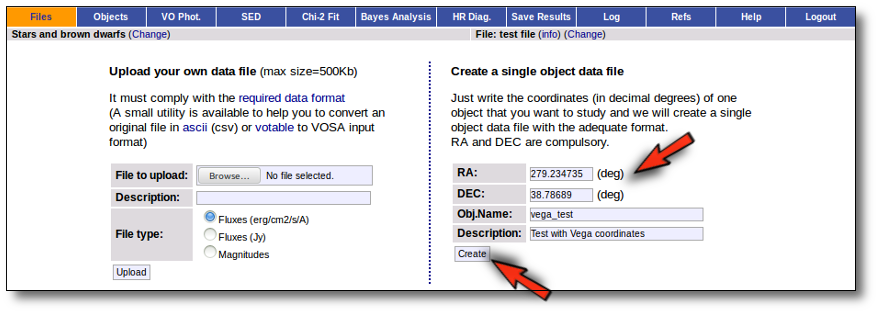
Single object search
In the case that you only want to work with a single object (or you just want to test how VOSA works) you don't need to build a input file.
You only need to specify the RA and DEC (in decimal degrees) of your objects. The object name and description are optional (if you leave any of them blank VOSA will fill them using the information in the other fields).
With those coordinates VOSA builds a very simple input file that is saved in your Default folder and you can then work with it, use VO catalogues to find out information or photometry for that object and then try to fit the observed SED with theoretical models.
Example
You only need to specify the RA and DEC (in decimal degrees) of your objects. The object name and description are optional (if you leave any of them blank VOSA will fill them using the information in the other fields).
With this information VOSA will make a very simple "VOSA input file" and it will be loaded automatically.
From then on, you will work with this file as with any other vosa file.
Just remember that the only information that we have for this object now is its coordinates. You will need, at least, to search for photometric data in VO catalogues using the "VO Phot." tab.
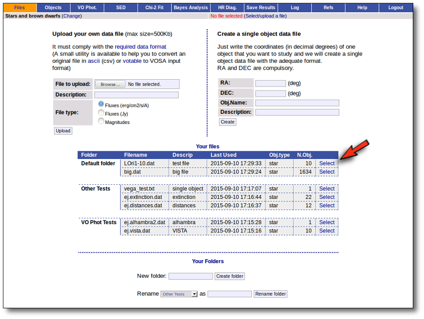
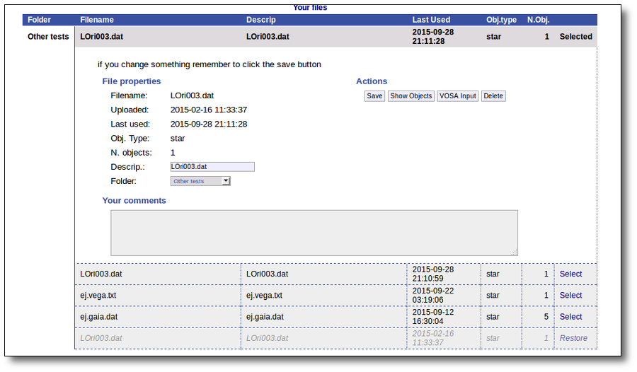
Managing your files
All the files that you upload to VOSA will be shown in the "Files" page.
You can organize them using folders. In the form in the bottom you can create folders as you like (or rename them).
To start working with VOSA You need to select one of the files.
For the selected file you can also:
- Edit the file description.
- Move it to another folder.
- Add comments (maybe to remember something about this file in the future).
In order to do that, you just need to edit that information in the form and click the "Save" button.
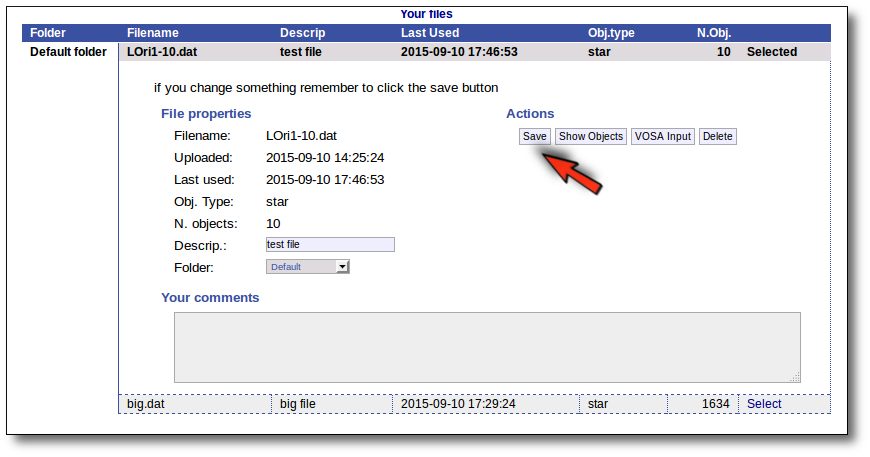
Click the "VOSA Input" button to recover the VOSA Input file that you first uploaded (you will get the same ascii file).

Click the "Show Objects" button to see the info about the objects in the file. Remember to do this after uploading the file to check that all the info has been understood by VOSA properly.
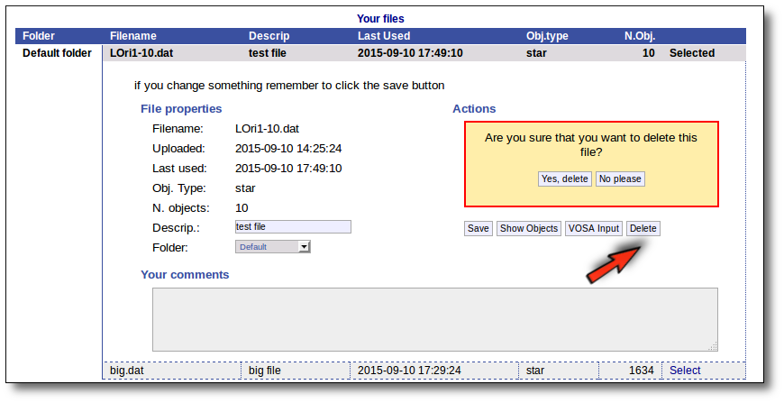
Click the "Delete" button to delete the file from VOSA (all the information about it will be lost). You will be asked for confirmation.
Archived files/Restore
Every file that you upload into VOSA is keeped in our server together with all the information related to every action that you do to the objects in that file (photometry, fit results, plots, etc.). You can come later and continue your work on any of your files at the point where you left it.
But if you haven't done any action on a file for 3 months we understand that you are not doing an active work on it and you do not really need it to be so easily accesible.
Thus, we archive files that have not been used in the last 3 months to save VOSA disk space and maintanaince.
Those files will be displayed in a different style in VOSA and you will not be able to select them directly.
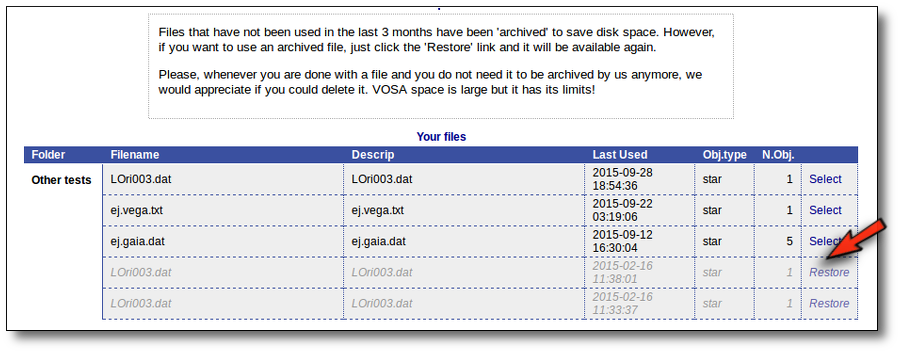
But if you really want to use that file again, you can click in the "Restore" link. VOSA will recover all the content so that you can work with it again.
The process will be almost inmediate for small files but could take a while if your file is big.
When everythink is ready you will see a message.

And when you click the "Continue" link, the content of your file will be available again.
In any case, please, whenever you are done with a file and you do not need it to be archived by us anymore, we would appreciate if you could delete it. VOSA space is large but it has its limits!
Available Filters
Most of the filters from the SVO Filter Profile Service are available to be used in VOSA using the FilterID as name.
Please, check the Filter Profile Service for details. The link will open in a different window.
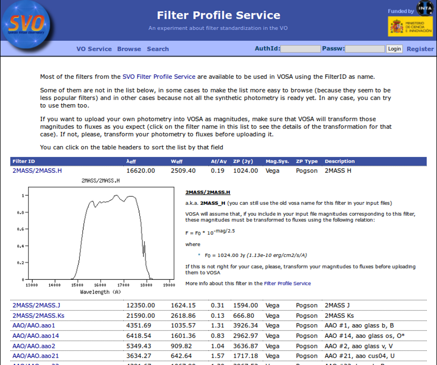
The filter properties are used by VOSA in a number of ways.
- The filter transmission curve is used to calculate the synthetic photometry for each of the available theoretical models or observational templates. This synthetic photometry is what will be compared to the observed photometry in the model fit or bayes analysis.
- The λeff will be used as the nominal value for the wavelength corresponding to the photometric point. This wavelength is used as follows:
- As the x coordinate for the different plots showing the object (or model) SED.
- To transform from Jy to erg/cm2/s/A if the original photometric values are given in Jy (either in your input file or in photometry coming from VO catalogs)
- Indirectly, the Af/AV value given by the FPS is calculated for this value of the filter wavelength. Thus, it has some effect in the deredenning.
- The zero point is used to transform magnitudes to fluxes if the original photometric values are given as magnitudes (either in your input file or in photometry coming from VO catalogs). In that case, the corresponding magnitud system will be taken also into account.
The link above shows a summary on how VOSA will use the filter properties. You can click on any filter name to see more details and you can also use the table column titles to sort the table using that field.
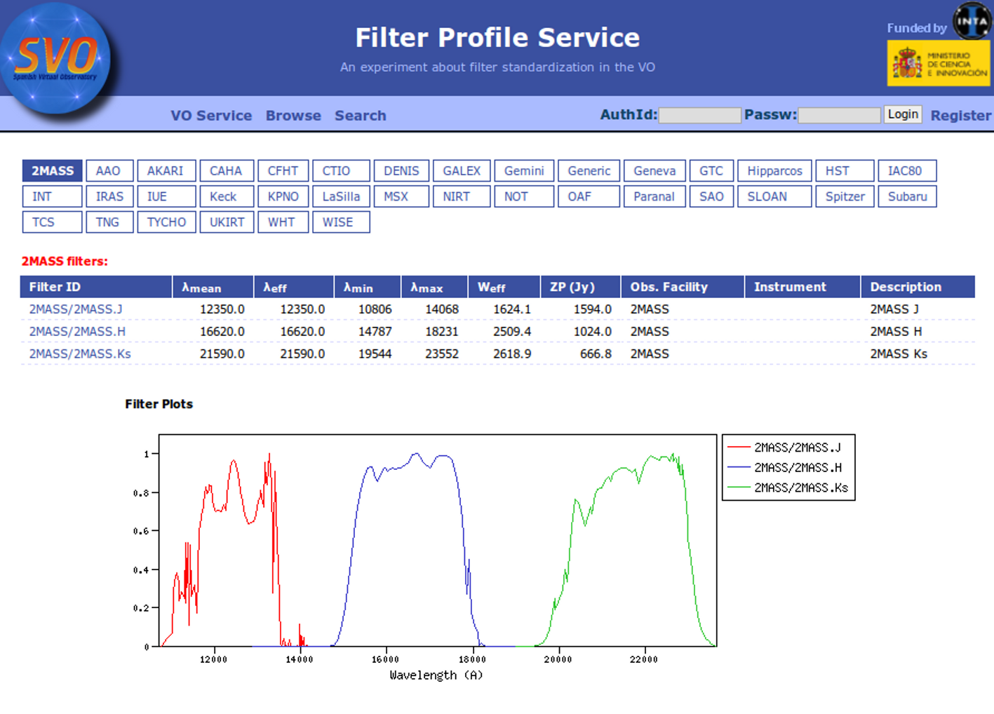
Besides that, you can access the full information in the Filter Profile Service using the "Browse" or "Search" links in the top menu. You can see a summary of all the filters in a given "family" (instrument, mission, survey, generic...) or click in any filter to see more details on the filter properties and how they are calculated by the service or where they were found in the literature.
Objects
There are some object properties that are important in order to be able to use all the potential of VOSA and get reliable results.
- Object coordinates are necessary to be able to make VO searches (for properties or photometry). Most operations in which we search for information in VO catalogs have to be made in terms of the object coordinates (and some search radius around them). If the coordinates are not available, you won't be able to search the VO.
- Object distance is necessary to be able to calculate bolumetric luminosities from the model fit results and then use these luminosities in the HR diagram to try to get estimation of the mass and age.
- The value of the visual extinction, Av, is necessary to deredden the observed photometry.
You can upload all this information in your Input file if you know it, but VOSA also can help to find values for these object properties searching in VO catalogs.
Object coordinates
VOSA offers the possibility of finding the coordinates of the objects in your user file.
Having the right coordinates for each object is necessary if you want to be able to search in VO services for object properties (distance, extinction) or photometry.
In order to do this, the object name is used to query the Sesame VO service.
Then you can choose to incorporate the found coordinates (if any) into your final data or not.
Take into account that this only will give proper results if the object name given in the user file is the real one. Otherwise either you will find nothing or the obtained coordinates will not have anything to do with the real ones and, if they are used to search for catalogue photometry, the obtained values (if any) will not really correspond to the object under consideration.
Two examples
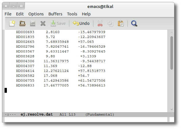
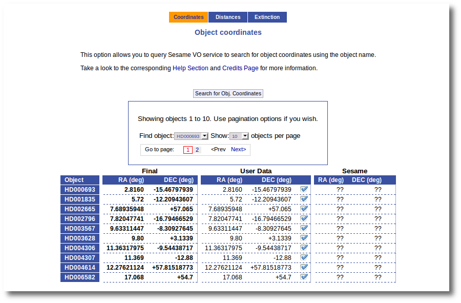
We upload a very simple file with some object names and no coordinates.
So the first thing that we do is clicking the button to "Search for Obj. Coordinates".
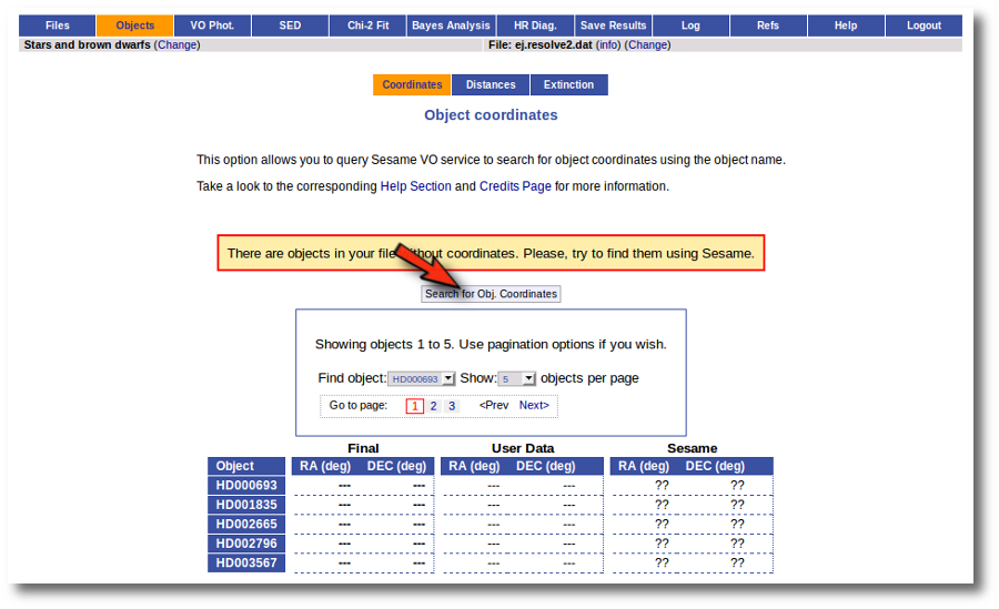
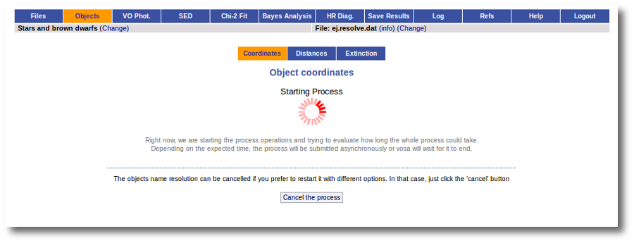
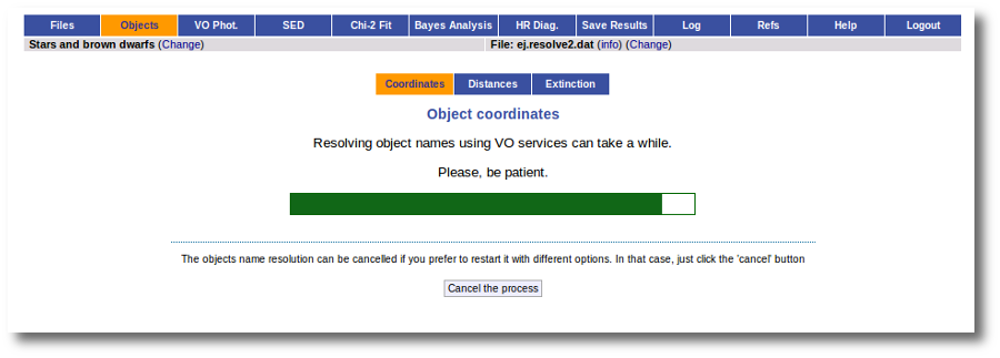
When you click the search button, VOSA starts the operation of querying Sesame for coordinates.
This search is performed asynchronously so that you don't need to stay in front of the computer waiting for the search results. You can close your browser and come back later. If the search is not finished, VOSA will give you some estimation of the status of the operation and the remaining time.
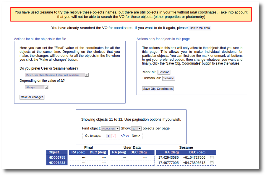
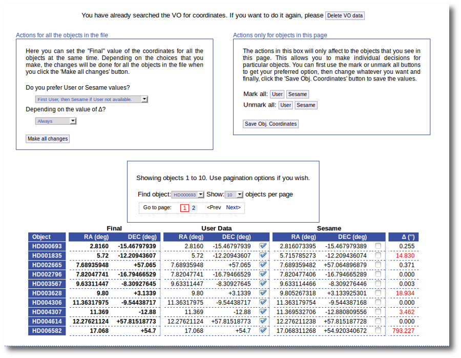
When the search is finished VOSA shows you the data obtained from Sesame, but these coordinates are not incorporated to the final data yet.
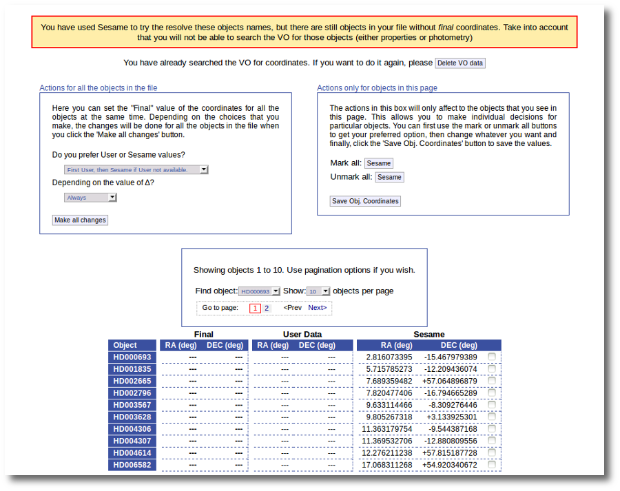
You have two different forms available. The one on the left allows to save data for all the objects in the file with a single click. The one on the right is useful to mark/save data corresponding ONLY to those objects that are displayed in the current page (not doing anything to objects in other pages, when there are many objects).
In this example we are going to use the form on the right.
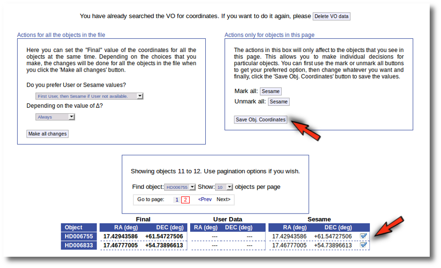
First we click the "Sesame" button so that all the values coming from Sesame are selected.
Then, we click the "Save Obj. Coordinates" so that the marked values get saved.
But we still see the warning saying that there are some objects without coordinates!
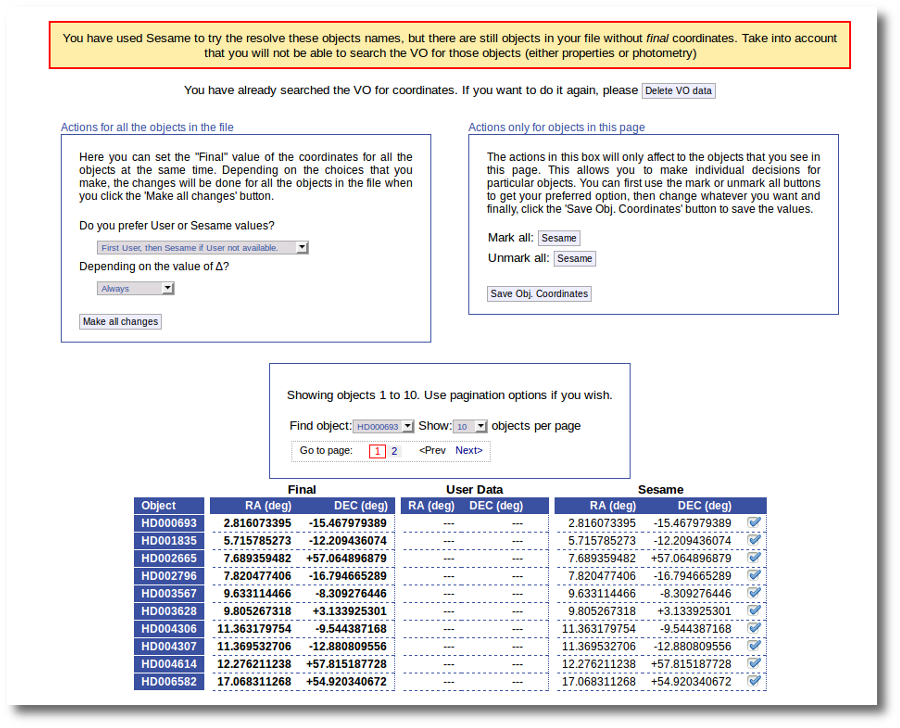
If we use the pagination form to go to that page we see that we haven't saved the distance for those objects yet.
In this case we just mark those two Sesame value by hand and click the "Save Obj. Coordinates" again.
Now he have the coordinates for all the objects in the file.
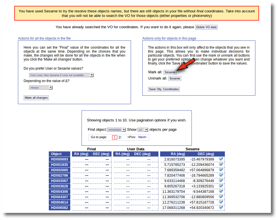
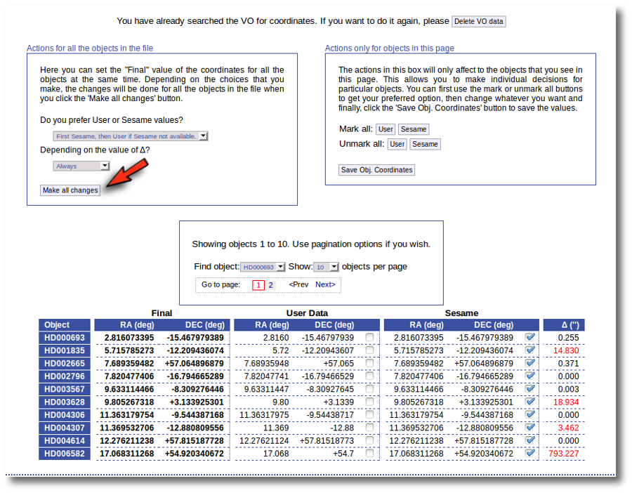
As a second example, we upload a file with the same objects but including RA and DEC values.
We can see the user values already selected and saved as final values.
We could stop here, but we want to check these coordinates comparing them with what we find in Sesame.
Thus, we click the "Search for Obj. Coordinates" button, we wait for the process to finish and we see, side by side, both user coordinates and Sesame values.
An extra column shows the difference, in arcsec, from the user coordinates and the sesame ones. This difference is shown in red when the difference is bigger than 1'' so that it is easier for you to discover suspicious cases.
In this example we use directly the form on the left. We select the option to use Sesame values values when available and to use them always. We click the "Make ail changes" button and Sesame values are directly saved as final for all the objects in the file.
Object distance
The distances to the objects are used by VOSA to transform the total fluxes given by the 'model fit' into bolumetric luminosities as:
Lbol = 4πD2 Ftot
If you don't give a value for the distance, VOSA will assume it to be 10pc to calculate the Luminosity.
If you don't care about the final luminosities and you don't intend to make an HR diagram, you can forget about distances and write them as "---" in your input file.
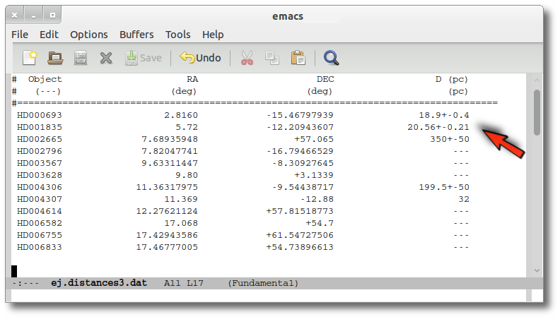
Distance errors
You can also provide a value for the error in the distance in your input file. In order to do that write D+-ΔD (for instance: 100+-20), without spaces, in the fourth column of your input file. See below for an example. (Remember to write both symbols, + and -, together, not a ± symbol or something else; otherwise vosa will not understand the value).
ΔD will be propagated as a component of ΔL as follows:
ΔLbol (from D) = Ftot * 2ΔD/D
If you don't give a value for ΔD or you don't find one in the VO, it will be zero. This will imply very small errors in ΔL as only errors coming from the observed fluxes will be considered.
VO search
VOSA offers the possibility of searching for the distance of the objects in VO catalogs.
In order to do this, the object coordinates are used to query some VO services (like Hipparcos catalog) to find observed parallaxes. Thus, object coordinates must be known (either provided in your input file or obtained in the Objects:Coordinates tab) if you want to search the VO for information about distances,
Take into account that the tool queries VO services using the object coordinates and returns the closer object to those coordinates, within the search radius, for each catalog. It could happen that the obtained information corresponds to a different object if the desired one is not in the catalog. In that case, the obtained distance could be erroneous because it corresponds to a different object. So, please, check the coordinates given by the catalog for each object to see if they seem to be the appropriate ones (within the catalog precision) before using the obtained values.
VOSA marks as "doubtful" those values found in catalogs so that the observed error is bigger than 10% of the parallax. It has been shown that for bigger errors the estimation of the distance from the parallax is biased (See Brown et al 1997). These values will be shown in red so that you are easily aware of large uncertainties.
The user can choose to incorporate the found distance (if any) into the final data or not. This decision can be taken in two different ways:
- Object by object. You can give user values for the distance (and error) for some particular objects, choose the value (user or VO catalogs) object by object, and just save those values.
- Specifying global criteria that will be applied to all the objects in the user file (which is specially useful for large files with many objects). Criteria are based on two main ideas: (1) what catalog you prefer to use and (2) the uncertainties for the distance values. See below for details.
Take a look to the corresponding Credits Page for more information about the VO catalogs used by VOSA.
An example
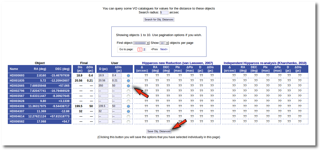
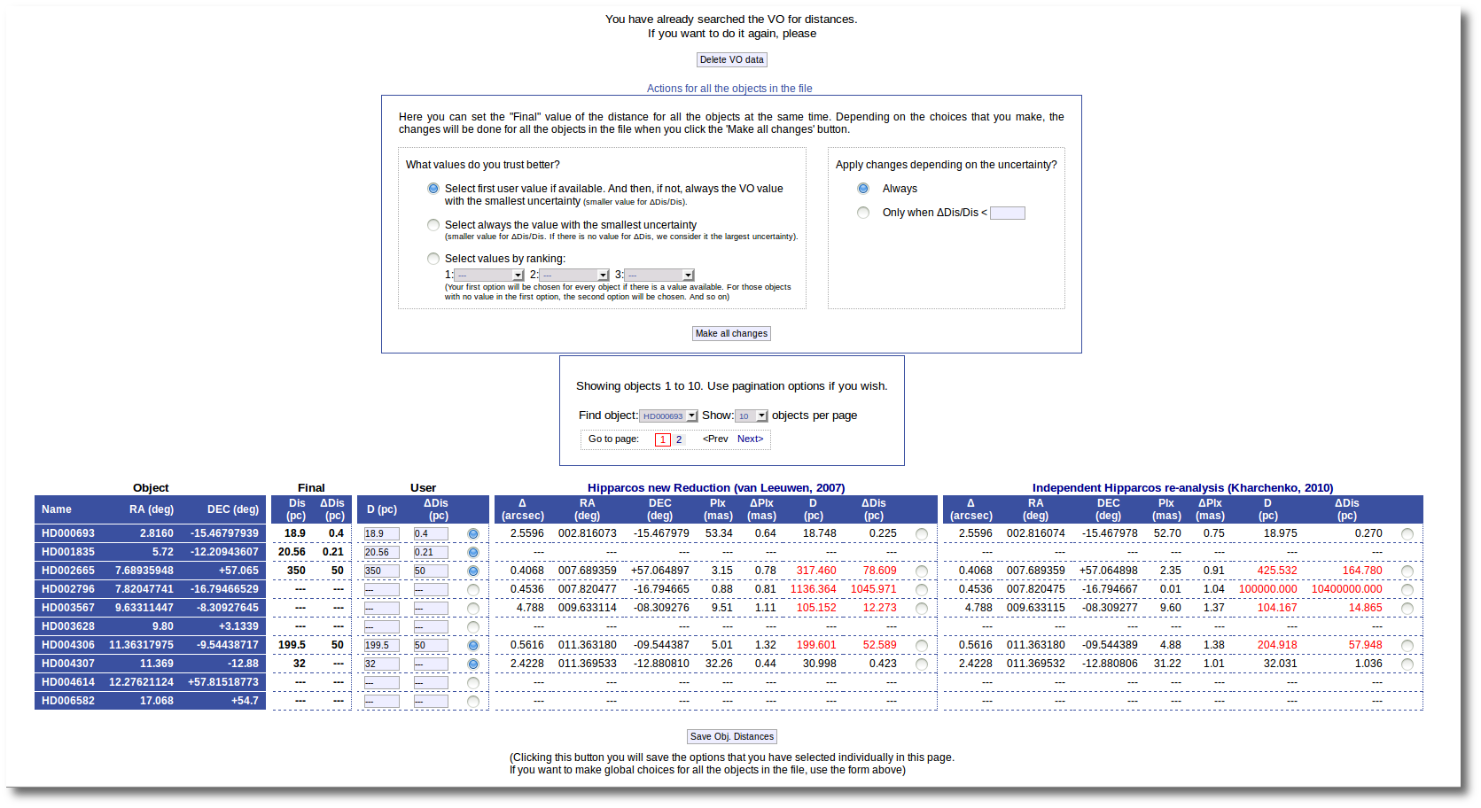
We have uploaded a file with information about the distance to some of the objects (in some cases we have included errors for the distance too). As you see we have values for distance and error for 4 objects, only the distance for HD004307 and no information about 7 objects.
We want to check the VO to search for more information, so we enter the Objects:Distances subtab to try to find something.
At this stage, we see three main functionalities:
- First, the possibility to search the VO.
- A pagination form (when there are more objects in the file than the number that you choose to visualize in each page).
- A form with the values of the distance for each object.
In this last form there are several groups of columns:
- Object information (object name, RA and DEC)
- The Final values. These are the values for the distance that will be used by VOSA outside this tab. In principle, the values here will be those values provided by you in your input file. But now you can change them.
- The User values. In principle, the values here will be those values provided by you in your input file. But now you can change them. And you can decide to used those new values as the final ones (or not).
- Information about the distance values found in VO catalogs for each object. At first this information is "unknown" because you haven't done a VO search yet.
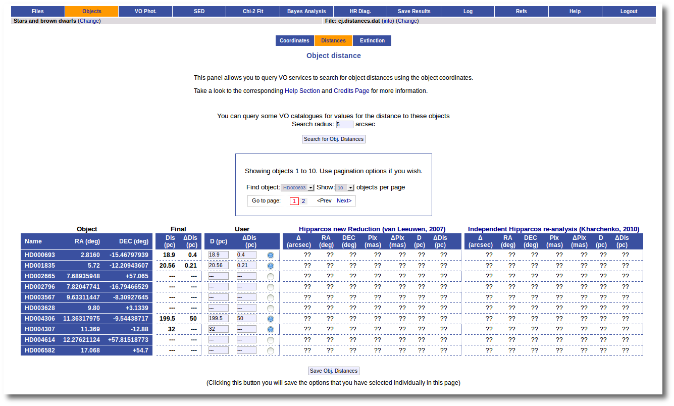
The first thing that you can do is editing the User values as you wish. For instance, you can give a value of 350±50 pc for the HD002665. You just need to write those values in the User column, mark the "tick" to its right and click the "Save Obj. Distances".
And you see that the final value for this object has been changed accordingly. If you leave this tab now, whenever a distance value is needed, VOSA will use a distance of 350±50 pc for this object.
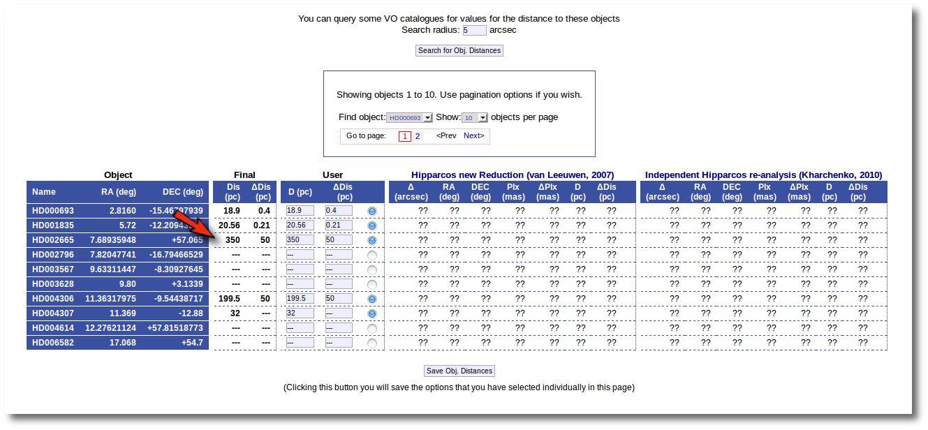
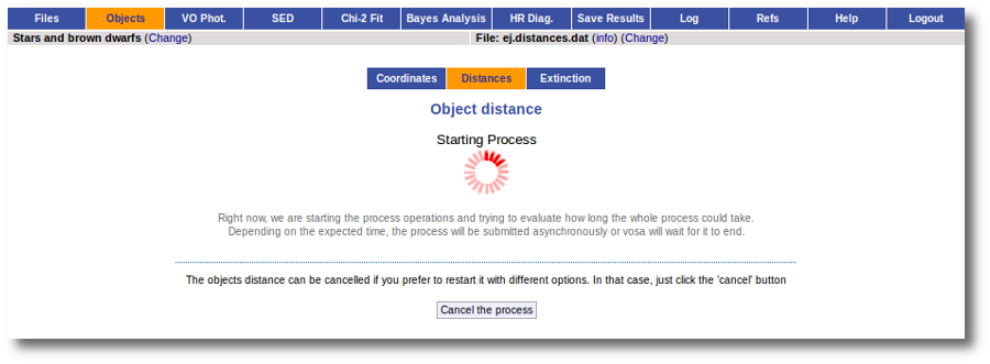
The next natural step is searching the VO for distance values. In order to to this you can just click the "Search for Obj. Distances".
When you click this button, VOSA starts the operation of querying VO catalogs.
This search is performed asynchronously so that you don't need to stay in front of the computer waiting for the search results. You can close your browser and come back later. If the search is not finished, VOSA will give you some estimation of the status of the operation and the remaining time.
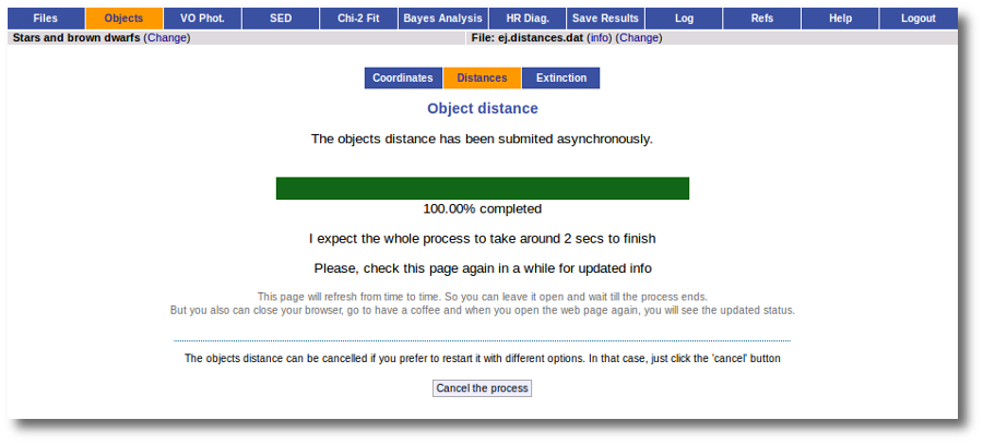
And, when everything is ready, you will see the values found in the VO catalogs for the distance to these objects.
Values with large relative errors are shown in red so that you are easily aware of large uncertainties.
At this point you still can choose to edit User values one by one and save them with the "Save Obj. Distances" button (as explained above). Or you also can decide to mark individually what value you prefer for each object among those available and click the "Save Obj. Distances" button to save those values as the final ones.
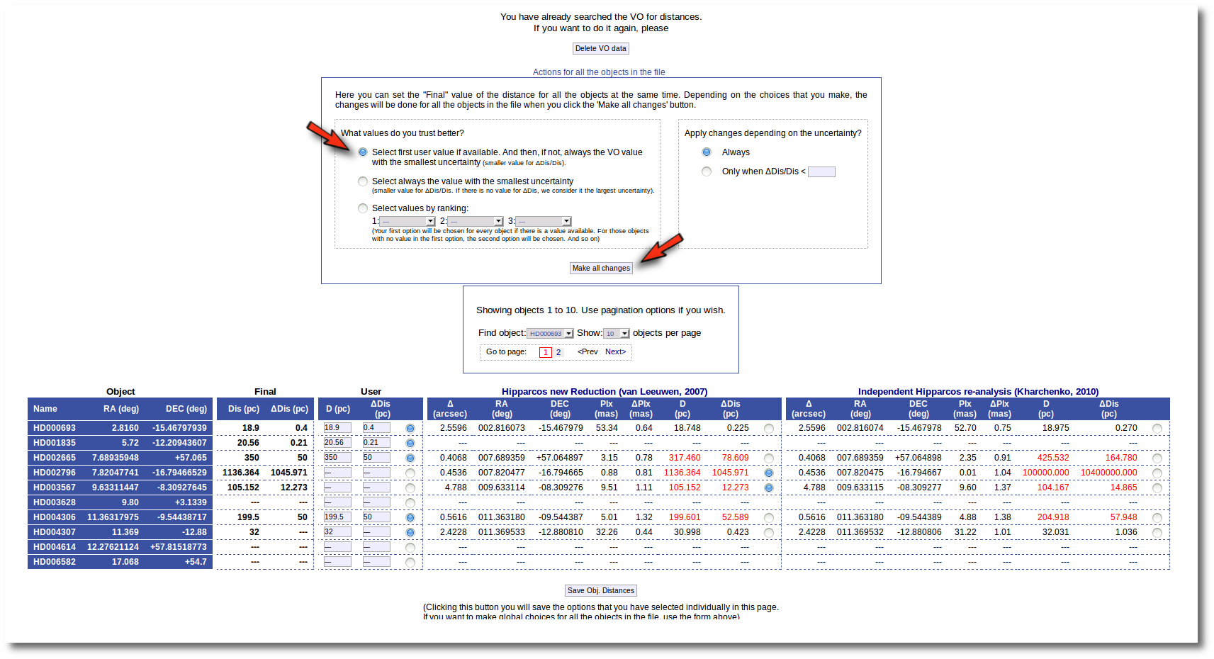
But you also can see a new form that offers you some options to choose the final values for all the objects in the file with just one click.
The form has two main parts:
- On the left, you have three different ways to prefer one catalog (or user values) over the other.
- Select first user value if available. And then, if not, always the VO value with the smallest uncertainty.
If you choose this, for those objects with user values, these will be chosen as the final ones. For those objects that don't have a user value for the distance, the one in VO catalogs with a smaller relative error will be saved as the final one. - Select always the value with the smallest uncertainty.
This means, quite obviously, that the value with a smaller relative error will be chosen. Take into account that if there is not a value for ΔDis, this will be considered as the largest uncertainty. - Select values by ranking.
Here you can specify the option that you prefer if there is a value available. If not, your second option will be used, and so on.
- Select first user value if available. And then, if not, always the VO value with the smallest uncertainty.
- On the right, you can decide if the above conditions are applied always or only when the relative error in the distance is below a certain limit. For instance, if you say that "Only when ΔDis/Dis < 0.5", if for one object, in one catalog, the relative error is larger, that will be considered as "there is not a value in this catalog".
When the "Make all changes" button is pressed, VOSA makes the selection adequate for your criteria and the corresponding values are saved as final.
For instance, if you mark the first option on the left, for those objects where is a value of the user distance, it will be the selected one, for the other objects, the van Leuween values are selected because they have smaller relative errors that the Kharcheko's ones.
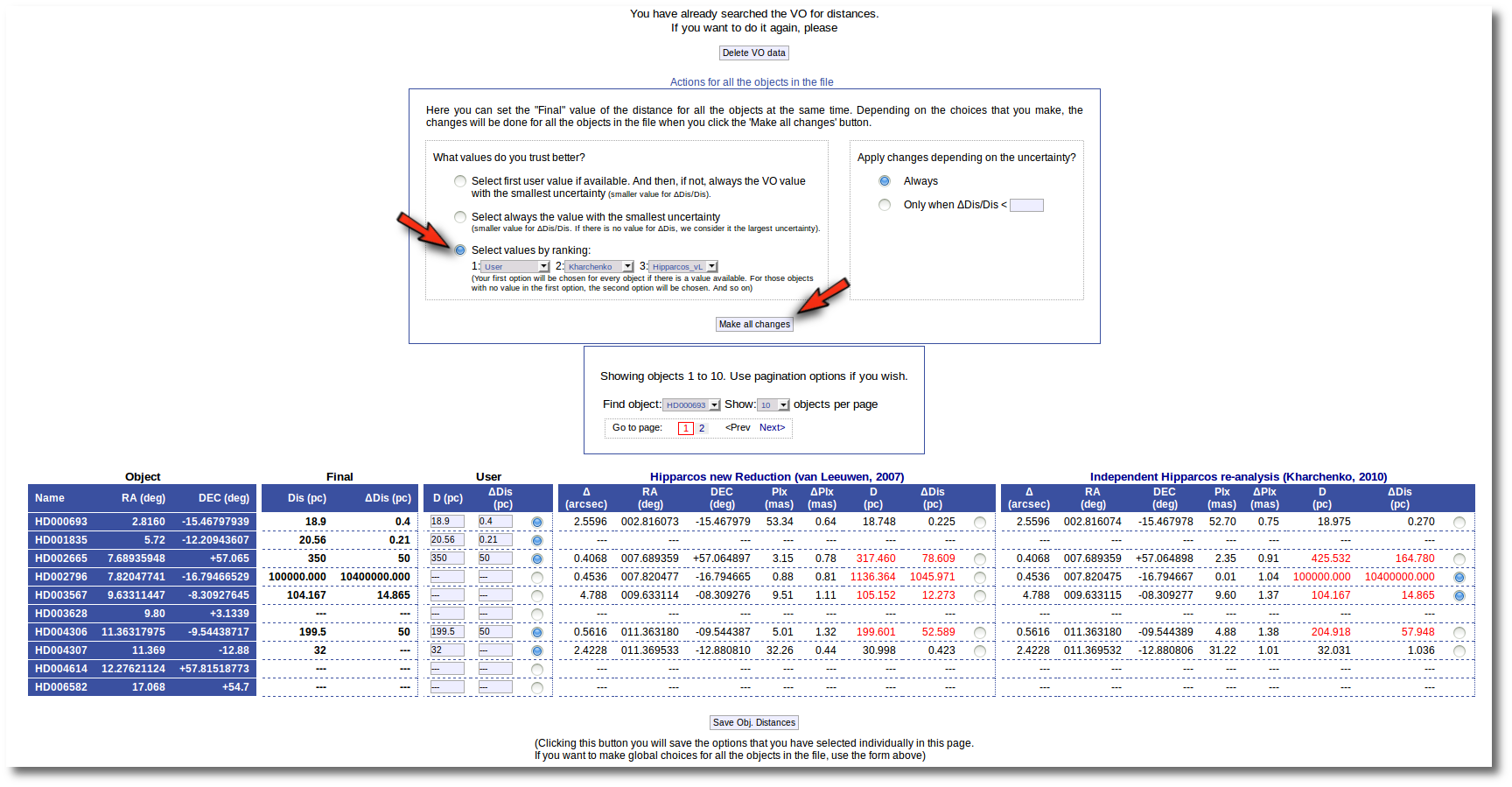
Then, we select the third option on the left. And we set our preferences as: (1) user, (2) Kharchenko, (3) van Leuween. When we press the "Make all changes" button, Kharchenko's values for the distance is selected for HD002796 and HD003567, because there is not a user value for those objects.
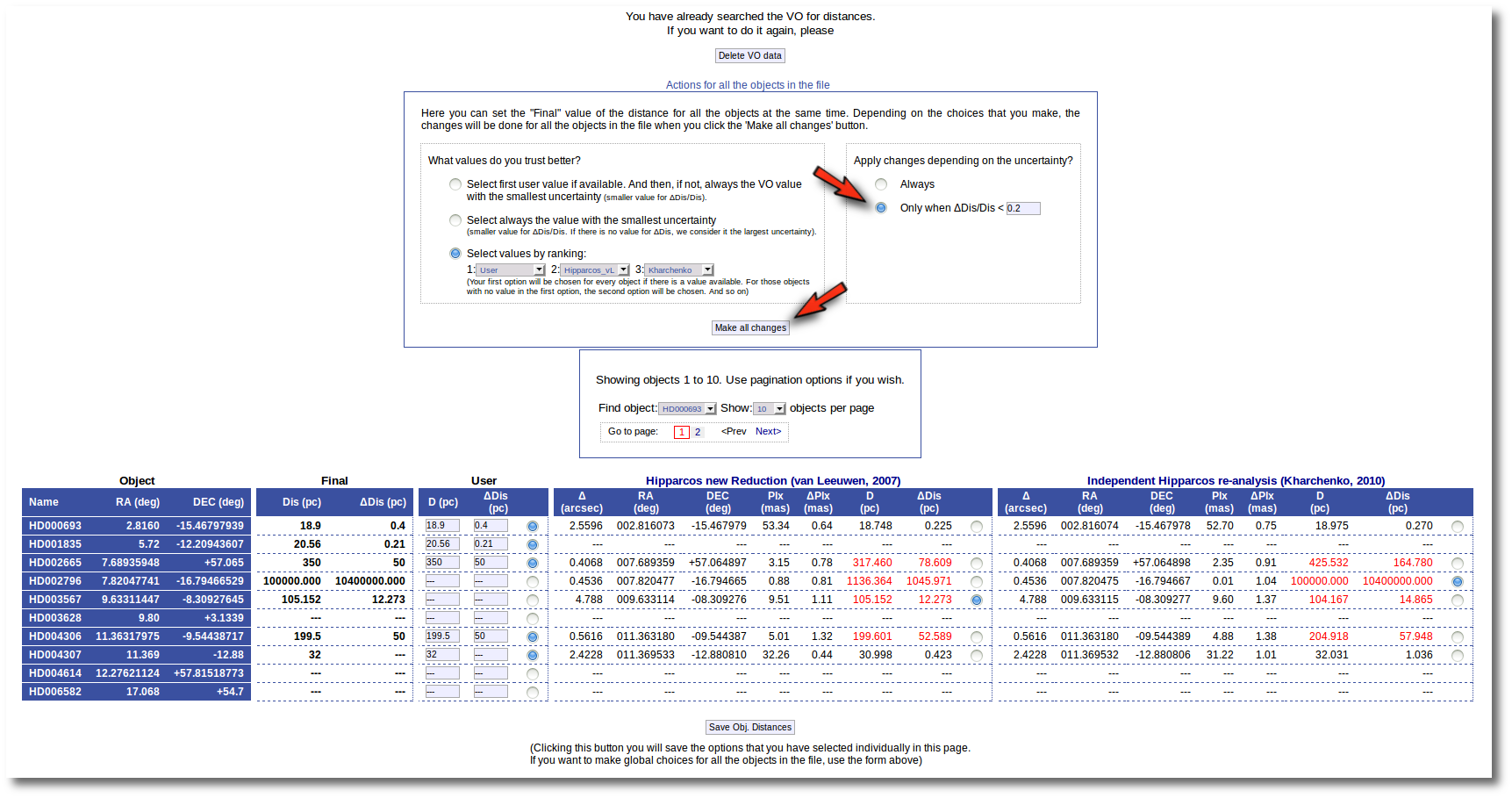
Then, we change the order of preference to: (1) user, (2) van Leuween (3), Kharchenko. And we also set a limit ΔDis/Dis < 0.2 to make changes. In this case, for HD003567 there is not user value, then the van Leuween one is considered and ΔDis/Dis = 0.116 so it is selected and saved. But for HD002796 ΔDis/Dis = 0.92 in van Leuween and ΔDis/Dis = 10,4 in Kharchenko. So none of the values is selected and no change is made: the final value is kept as it previously was.
Extinction
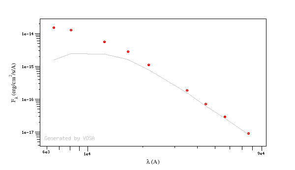
The value of the interestellar extinction is necessary to deredden the observed photometry before analyzing it. If the extinction is not negligible, the shape of the real SED can be very different from the real one and any physical property estimated using the SED, if not properly unreddened, can be erroneous.
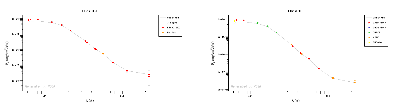
For instance, see the difference the observed SED (gray line) and the dereddened one (red points) for an object with Av=3.
You can provide a value for the visual extinction Av for each object in your Input file. But, if you don't have those values, VOSA also offers the posibility to search VO catalogs for extinction properties.
And, finally, you can also give a range of values for Av so that the model fits (chi2 and bayes) fits together the model physical parameters and the value for Av.
The extinction law.
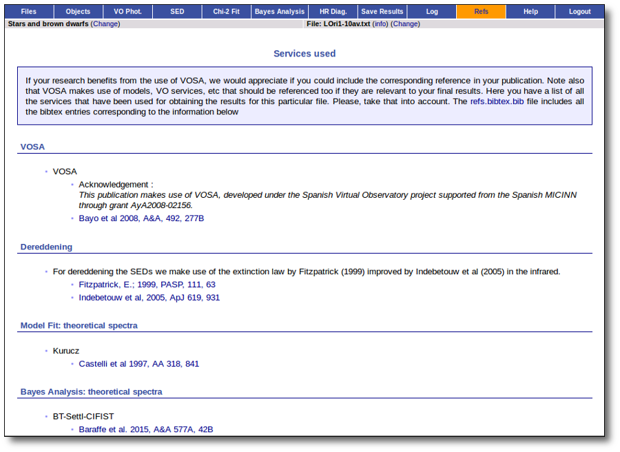
For dereddening the SEDs we make use of the extinction law by Fitzpatrick (1999) improved by Indebetouw et al (2005) in the infrared. Take a look to the corresponding Credits Page for more information.
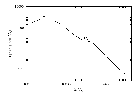
(You can download the tabulated data for the extinction law).
The extinction at each wavelength is calculated as: Aλ = AV * kλ/kV, where kλ is the opacity for a given λ and kV=211.4
VO extinction properties.
The tool offers the possibility of finding extinction properties of the objects in the user file.
In order to do this, the object coordinates are used to query some VO services to find AV or RV and E(B-V) for each object.
Then you can choose to incorporate the found values (if any) into the final data or not. In fact, if it happens that diffferent catalogues give different information about the relevant quantities, you can choose which data to use to build the final AV value.
Remember that, if you decide to save new values for AV, the original data will have to be deredden again using the new values. This will change the final SED and, thus, if any other analysis has been done for the corresponding SED (for instance, a model fit) this analysis will have to be done again.
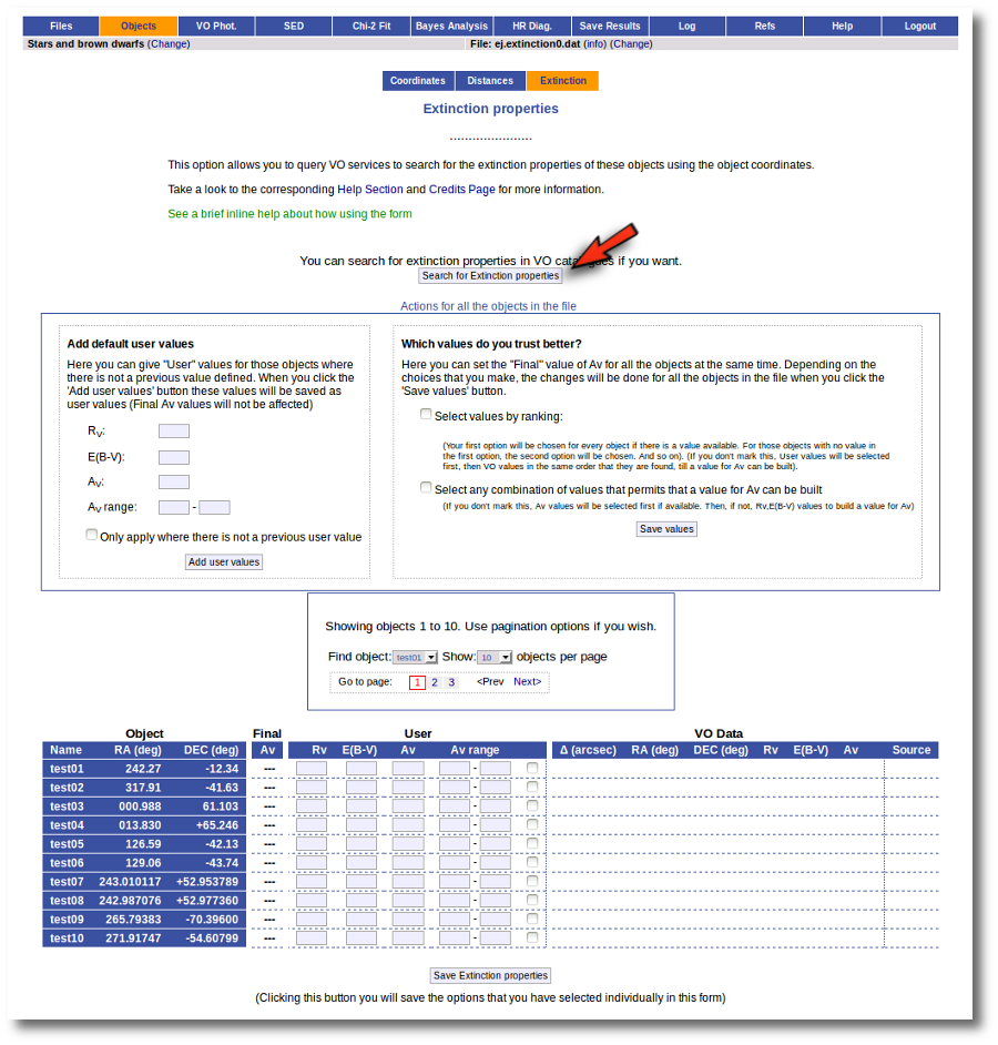
The first time that you enter this section for a given input file, the tool shows the AV values given in the input file (if any) and a button to search into VO services. When a search has been done, the tool will show the user values together with the found values for each relevant quantity so that you can choose which ones should be used (checking the corresponding box).
In fact, this form has several options that can be combined. Take into account that
- Some VO catalogues provide AV directly, but other catalogues give information about RV or E(B-V). Using RV and E(B-V), AV can be calculated as AV = RV * E(B-V).
- VOSA can combine the data given by you in your input file and the information found in VO catalogues.
- You can write default values for AV, RV, E(B-V) or the AV range to be used in the fits. If you do so, click the 'Add user values' button to fill the corresponding User columns with those values (only if there is not a previously saved value).
- Click the 'Search for extinction properties' button for seaching several VO catalogues.
- For each object, if you want to save some information, check the corresponding checkbox. If you mark values for RV and E(B-V) they will be used to calculate AV. If you want to do so, mark the ticks with the values that you want to save, and click the 'Save extinction properties button' and the AV values will be saved and shown in the 'Final' column (if there was enough information).
- When you have a large list of objects, it is difficult to do this object by object. You can also give some general criteria about what catalog information you trust better, and let VOSA try to build Av values for all the objects in the file using the available information. See below for a detailed example on how to use the different forms.
Take into account that the tool queries VO services using the object coordinates and returns the closer object to those coordinates for each catalogue in a given search radius. It could happen that the obtained information corresponds to a different object if the desired one is not in the catalogue. In that case, the obtained data could be erroneus, as it corresponds to a different object. So, please, check the coordinates given by the catalogue for each object to see if they seem to be the appropiate ones (within the catalogue precision) before using the obtained values.
Take a look to the corresponding Credits Page for more information about the VO catalogues used by VOSA.
An example
We have uploaded a file with some objects and their coordinates, but we don't have information about the extinction for each object.
Thus, when we enter the "Objects:Extinction" tab in VOSA we see the list of objects and no extinction properties. We also see some forms:
- A button to seach the VO for extinction properties.
- A box, on the left, where we can add default values for AV, RV, E(B-V) or the AV range to be used later in the fits.
- A box, on the right, where we can give some criteria about our preferences among catalogs (this is of no use yet because we still don't have any information).
- A pagination form to see all the objects page by page.
- A "Save extinction properties" button that would be useful to save particular values for only the objects that we can see in the page.
We will see all these options with some detail below.
But, given that we don't have any information, our first step is searching for these objects in VO catalogs. And, thus, we click the "Search for extinction properties" button.
We get a list of all the catalogs that VOSA can use to search for VO properties. You can leave it as it is and just click the "Search" button. But you also could unmark some of them if you know, for some reason, that they are not going to be useful. You also can change the default Search Radius for some catalogs if you are aware that a differrent radius is more adequeate for your case.
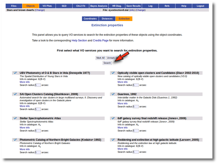
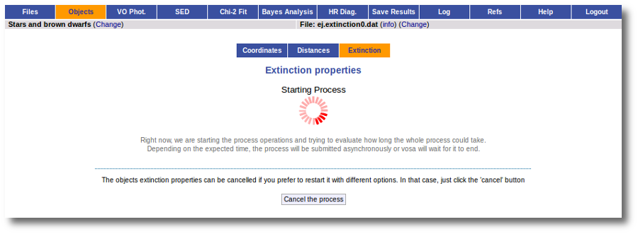
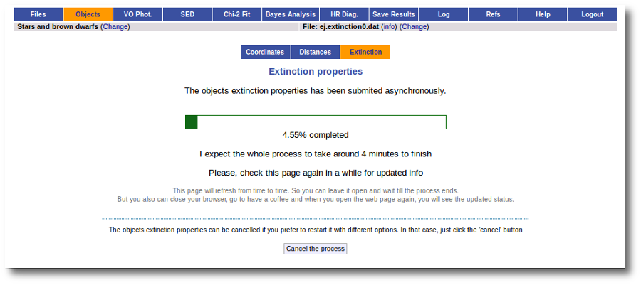
We just click "Search". When we click this button, VOSA starts the operation of querying VO catalogs.
This search is performed asynchronously so that you don't need to stay in front of the computer waiting for the search results. You can close your browser and come back later. If the search is not finished, VOSA will give you some estimation of the status of the operation and the remaining time.
When the search is finished, VOSA shows you, on the right, all the information that has been found for each object. In some cases, we don't get any information at all (for instance, for objects 'test01' and 'test02'). In other cases we only get information from one catalog. But in some cases (for instance, objects 'test03' and 'test04') we get heterogeneus information from more than one catalog.
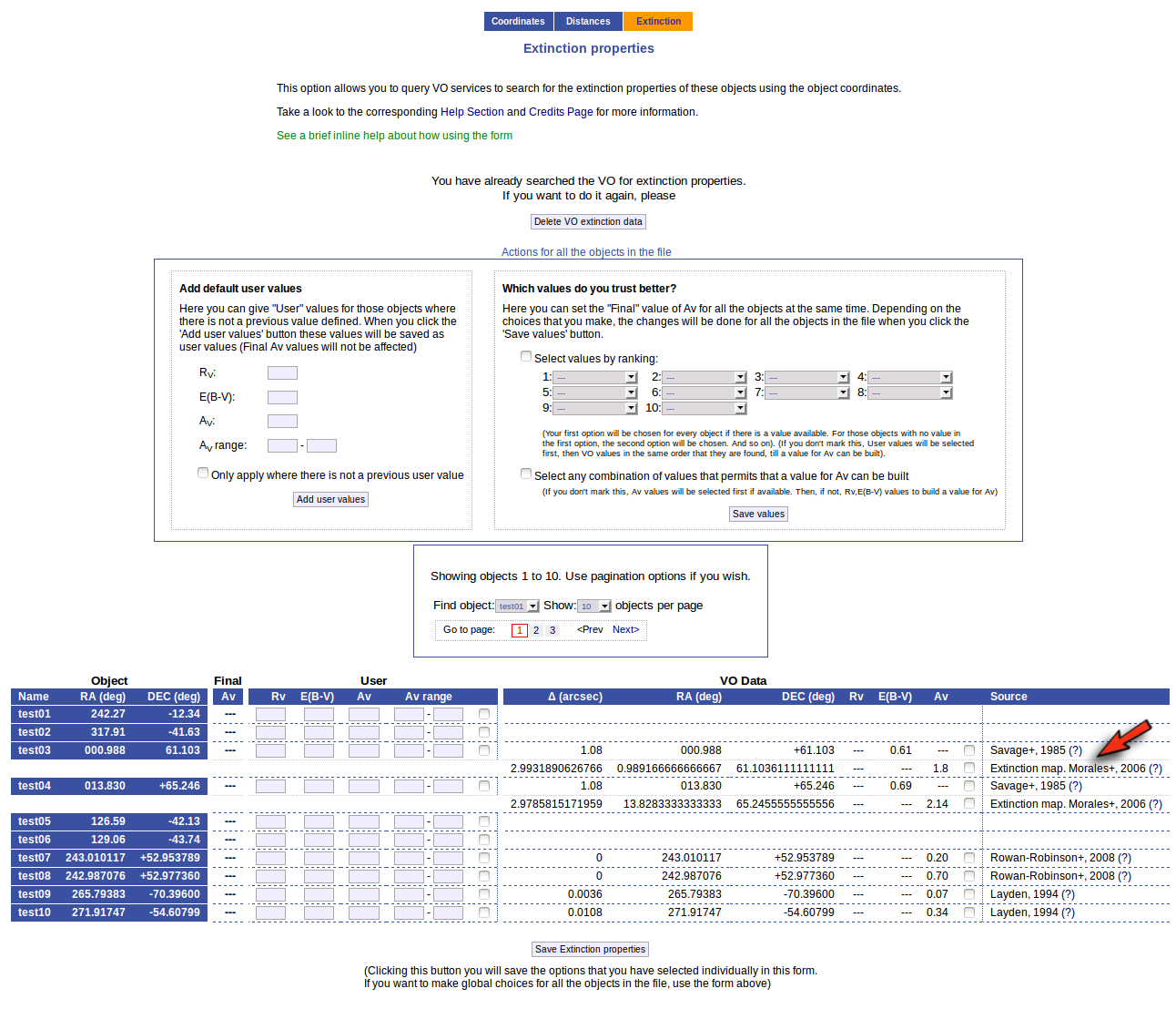
It happens very often that catalogs give values for E(B-V) but not for Av (like the Savage one in this example) and we need a value of RV to calculate AV using the expression AV=RV * E(B-V).
Thus, our first action is going to be adding 'Default user values' for some quantities. We write a value RV=3.1 in the "Default User Values" form and also a default fit range of (0-1) for Av. Then we click in the "Add user values" button (we could write the RV in the "User" column, object by object, but it's easier to do it this way).
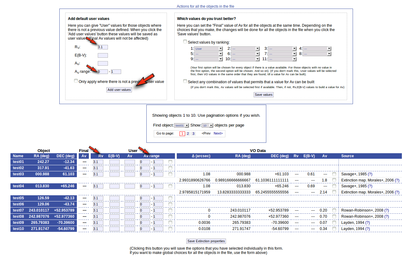
Now we have values for RV so that VOSA can use them if they are necessary to build a AV value for some object.
Next, we use the form on the right to let VOSA try to build values for Av for all the objects. We mark the tick correspoding to "Select any combination of values that permits that a value for Av can be built" and click the "Save values" button.
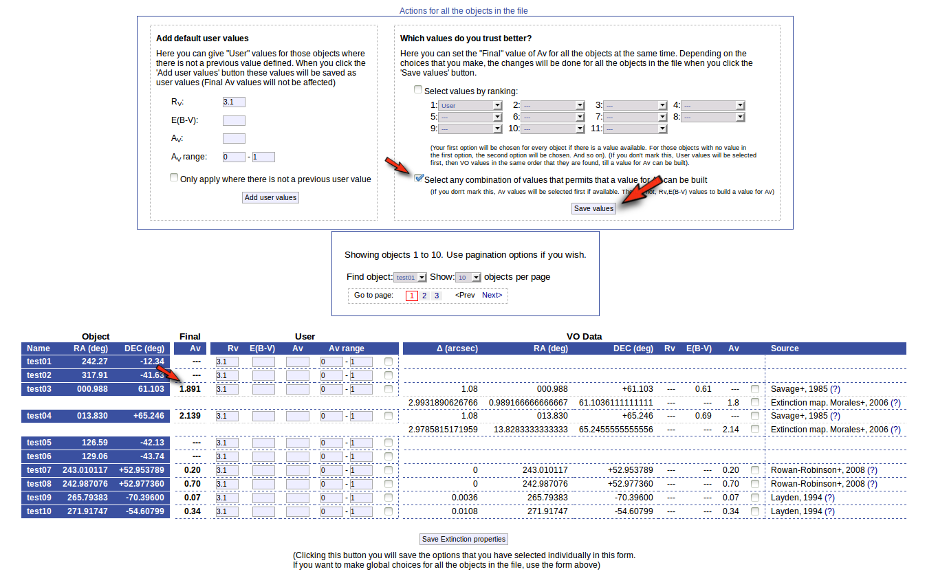
As you can see:
- For objects 'test01' and 'test02' nothing can be done, because there isn't enough information available, and nothing has been changed.
- For objects 'test07' to 'test10' it has been easy. There is only information from one catalog for each object. And in every case the catalg gives a value for Av. Thus, this is set as the final value of Av for those objects.
- For objects 'test03' and 'test04' there are two different options that can be used to build a value for Av. VOSA always chooses the first combination of values that allows for calculating Av. Thus:
- For 'test03', VOSA first tries E(B-V)=0.61 from Savage and, given that we have a default value Rv=3.1, a value Av=3.1*0.61=1.891 is calculated and saved.
- For 'test04', VOSA first tries E(B-V)=0.69 from Savage and, given that we have a default value Rv=3.1, a value Av=3.1*0.69=2.139 is calculated and saved.
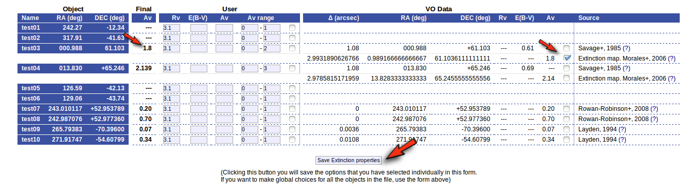
But we decide that we prefer Av=1.8 (from Morales) for the object 'test03' instead of the 1.891 value calculated before. And we want to make that particular change only.
Thus, we go to the list and:
- We mark the tick corresponding to the Morales catalog for 'test03' so that it is the value saved as final.
- We then click the 'Save Extinction properties' button.
and the 1.8 value is set as the final one for 'test03'.
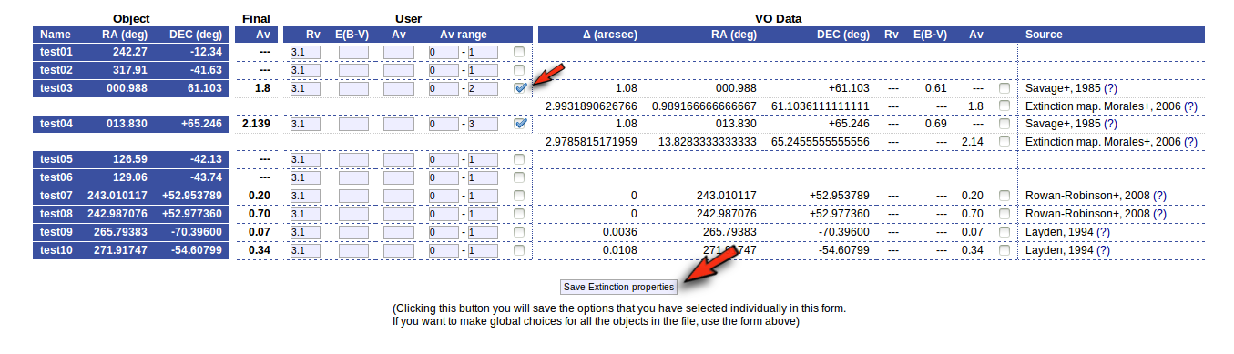
But then we notice that, given that for objects 'test03' and 'test04' we have Av values 1.8 and 2.139 it does not make sense that, later, when performing model fits, we try an Av range between 0 and 1. We set that default range before, when we didn't have any information, but now we should change that range, at least, for these two objects.
Thus, we go to the list and make these changes one by one.
- We set Av range = 0-2 for 'test03' and mark the tick on its right.
- We set Av range = 0-3 for 'test04' and mark the tick on its right.
- We then click the 'Save Extinction properties' button.
And the Av fit ranges are changed only for these two objects.
Build SEDs
VOSA helps you to build and/or improve the observed Spectral Energy Distribution (SED) for the objects in your file in different ways.
First, you can upload your own photometry into VOSA for each object including it in your input file.
If you include your data as magnitudes or Jy, VOSA will transform them into erg/cm2/s/A using the information for each filter provided by the SVO Filter Profile Service.
You can search in VO catalogs to find more photometry for your objects and those new points (if any) will be included in your objects SED. Again, if the catalogs provide data as magnitudes or Jy, VOSA will transform them into erg/cm2/s/A using the information for each filter provided by the SVO Filter Profile Service.
In the case that, for an object, there are several photometry values corresponding to the same filter but coming from different sources (user and VO, different VO catalogs, same source at different epochs...) VOSA will average them and include the average value in the final SED.
Every observed SED will be dereddened using the value for Av provided by you in your input file or in the "Objects:Extinction" tab (with the option of searching VO catalogs for extinction properties).
For each object, VOSA will try to detect the presence of infrared excess using an automatic algorithm.
Then you have the option to inspect (and optionally edit) the final SED object by object.
VO photometry
Search for photometry in VO catalogues.
The tool offers the possibility of searching in the VO for catalog photometry for the objects in the user file.
In order to do that, the object coordinates must be known as precisely as possible. Either the user can provide these coordinates in the input file or they can be obtained also from the VO.
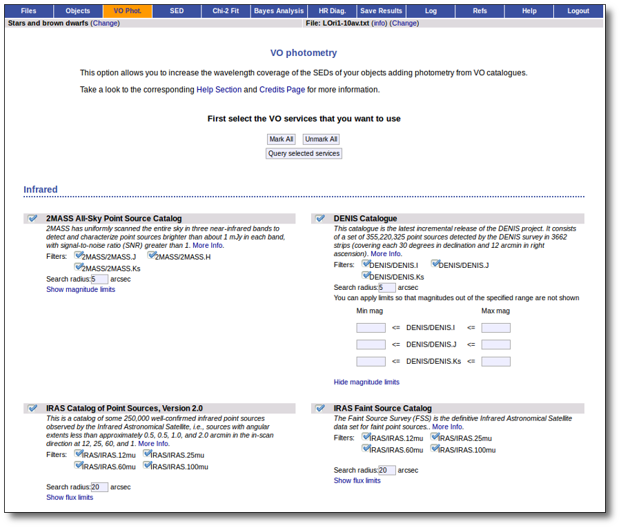
VOSA offers access to several catalogs with observed photometry from the infrared to the ultraviolet.
You can choose which catalogs to use and the search radius within each one.
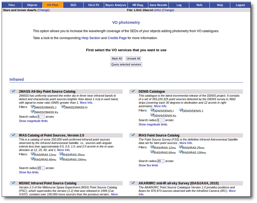
For each catalog, you have the option to establish magnitude limits, so that only photometry values in that range will be retrieved.
For each object in the user file, each catalog will be queried specifying the given radius, and the best result (the one closer to the object coordinates) will be retrieved. For some catalogs there are special restrictions. For instance, for the UKIDSS surveys, the search is restricted to class -1 (star) or -2 (probable star) objects. These special restrictions, when applied, are explicitly commented in the brief catalog description in the VOSA form.
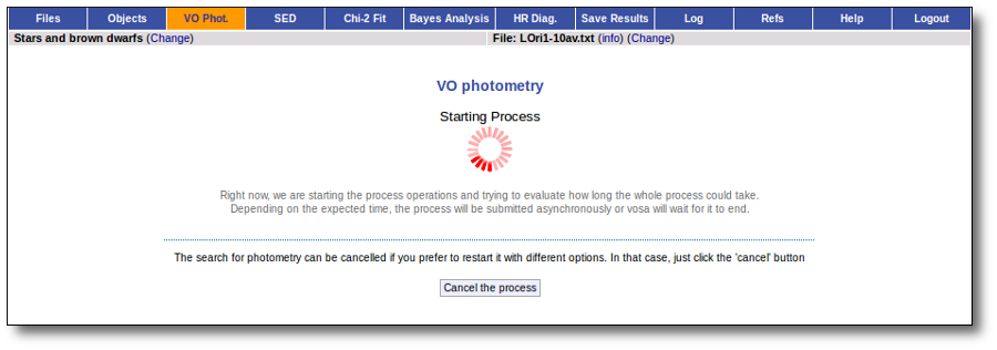
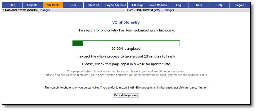
When you click the "Search" button, VOSA starts the operation of querying VO catalogs.
This search is performed asynchronously so that you don't need to stay in front of the computer waiting for the search results. You can close your browser and come back later. If the search is not finished, VOSA will give you some estimation of the status of the operation and the remaining time.
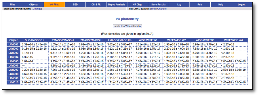
When the search process is finished you will see the photometric values obtained for each object (if any).
If the catalog provides magnitude values, these are automatically converted to fluxes.
Take a look to the Credits section for information about the available VO catalogs.
Detection of outliers in VO data
When new data are found in VO catalogues and before incorporating them to the object SED, VOSA tries to identify the presence of outliers, that is, photometric points that, for one or another reason, seem not to be part of the real SED.
In particular, VOSA looks for V patterns and inverted V patterns, that is:
V pattern
VOSA looks for points that seem to be clearly below the main SED, that is points so that both the previous and next points have much higher fluxes. To be more precise, if all these criteria are met:
- Fn-1/Fn > 5
- Fn+1/Fn > 5
- λn-λn-1 < 2500A
- λn+1-λn < 2500A
Although in the infrared, when 10000> ≤ λn-1 ≤ λn < 26000A, the criteria above is changed to: - λn-λn-1 < 6000A
- λn+1-λn+1 < 6000A
the point (λn,Fn) is considered suspicious and thus is marked as 'bad'. A 'lowflux' flag will also be included in the vosa and SED files if they are downloaded later.
Take into account that to make these calculations only the points (both from VO catalogues or User data) that are not flagged as 'bad' or 'upper limit' will be considered.
A simple example can be seen in this image:
We can see a first suspicious point for CTIO/DECam.g:
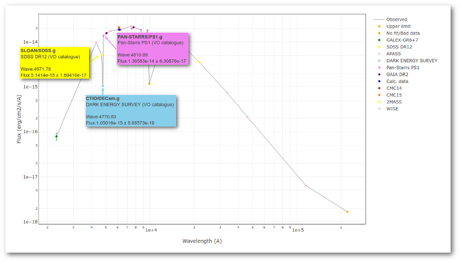
But VOSA will not flag it as bad because it does not meet the criteria
- Fn-1/Fn = 5.141e-15/1.050e-15 = 4.89 < 5
- Fn+1/Fn = 1.366e-14/1.050e-15 = 13.00 > 5
- λn-λn-1 = 4770.83 - 4671.78 = 99.05 < 2500A
- λn+1-λn = 4810.88 - 4770.83 = 40.05 < 2500A
But the point for CTIO/DECam.Y will be marked as bad:
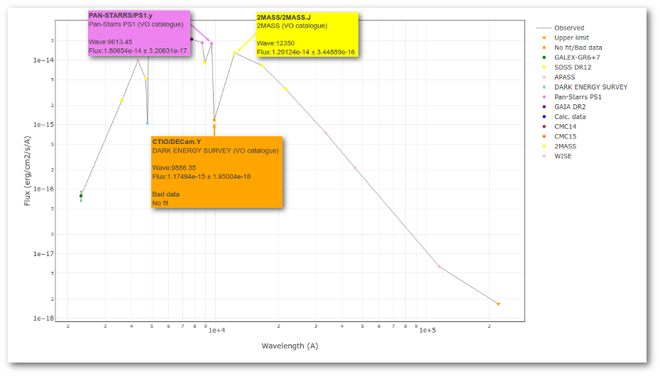
- Fn-1/Fn = 1.807e-14/1.175e-15 = 15.37 > 5
- Fn+1/Fn = 1.291e-14/1.175e-15 = 10.98 > 5
- λn-λn-1 = 9886.35 - 9613.45 = 272.9 < 2500A
- λn+1-λn = 12350 - 9886.35 = 2463.65 < 2500A
because all the criteria are met.
Inverse V pattern
VOSA looks for points that seem to be clearly above the main SED, that is points so that both the previous and next points have much lower fluxes. To be more precise, if all these criteria are met:
- Fn/Fn-1 > 5
- Fn/Fn+1 > 5
- λn-λn-1 < 2500A
- λn+1-λn < 2500A
the point (λn,Fn) is considered suspicious and thus is marked as 'bad'. A 'highflux' flag will also be included in the vosa and SED files if they are downloaded later.
Take into account that to make these calculations only the points (both from VO catalogues or User data) that are not flagged as 'bad' or 'upper limit' will be considered.
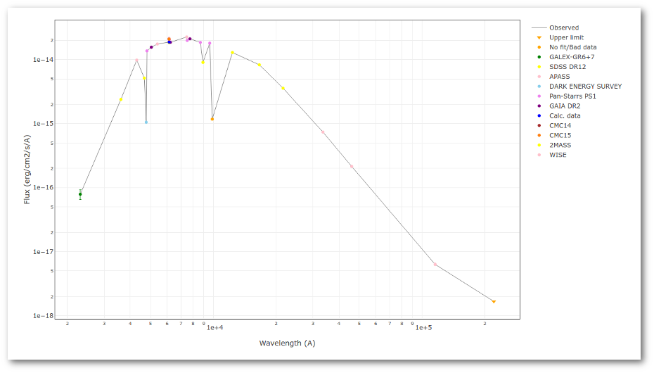
A simple example can be seen in this image:
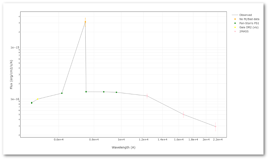
The point for will be marked as bad:
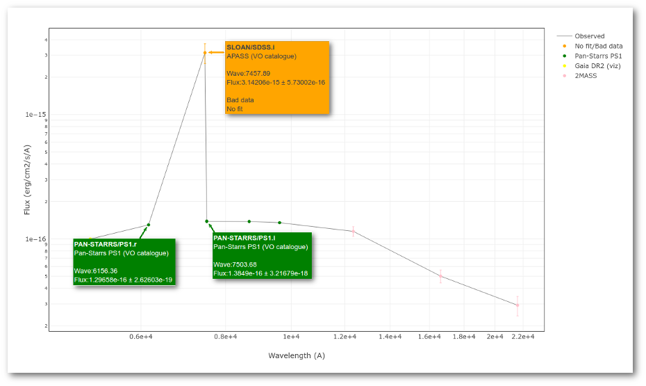
- Fn/Fn-1 = 3.142e-15/1.297e-16 = 24.22 > 5
- Fn/Fn+1 = 3.142e-15/1.385e-16 = 22.68 > 5
- λn-λn-1 = 7457.89 - 6156.36 = 1301.53 < 2500A
- λn+1-λn = 7503.68 - 7457.89 = 45.79 < 2500A
Object SED
VOSA helps to build a Spectral Energy Distribution (SED) for each object in the file combining user input data with data obtained from VO catalogues, taking into account extinction properties for deredening the observed fluxes and marking photometric points where IR or UV excess is detected.
In the SED section of VOSA you can visualize how the final SED has been built, what points have been considered, where the photometric points come from (VO catalogue, user input, etc), some properties of the data when coming from VO catalogues (including data quality when available) and, finally, where an IR excess has been detected by VOSA.
You can also edit the final SED and make decisions about what points are considered and how they enter the final SED. This is specially tricky when there are different photometric values for the same filter (coming from the user input file and/or VO catalogues).
Point options and actions
There are some options that allow you to decide how the final SED is built:
- Delete: Be careful. If you mark the 'Delete' checkbox for any point and then click the 'Apply Changes' button, this point will be deleted from the SED without confirmation. And you will not be able to undo the operation. So please, be careful.
- Ignore: If you mark the 'Ignore' checkbox for a point, this point will be ignored. It is as if it is deleted but it will be there so that you can recover it later if you want. It will not be part of the final SED, it will not be considered to make averages if there are more points for the same filter, it will not be shown in the SED plots...
- Nofit: Points marked as 'nofit' will be considered for the final SED but they will not be used in the model fits (chi-square or bayes). The point will be shown in plots in a different color.
- Uplim: Points marked as 'uplim' are assumed to be upper limits, not actual photometric values. But remember that VOSA does not really consider upper limits in the fits. These points will be authomatically marked as 'nofit' too. They will be shown in plots in a different color and they won't be used for the fits.
- Bad: Points marked as 'bad' are assumed to be points with bad quality for whatever reason. They will be marked as 'nofit' too. In some cases VOSA authomatically marks a VO photometry point as 'bad' when we know how to detect 'bad quality' in that particular VO catalogue.
Several values for the same filter
In some cases it happens that there are several observed photometric values for the same filter. For instance, if you have given a value for one filter in your input file and another value is found, for the same filter, in a VO catalogue.
When this happens, VOSA will calculate an average of the different values and this average is the value that goes to the final SED.
The average is calculated as: $$ \overline{F}=\frac {\sum ( {\rm F}_{\rm i}/\Delta{\rm F}_{\rm i} )}{\sum ( {1}/\Delta{\rm F}_{\rm i} )}$$ $$\Delta\overline{F} = \sqrt{\sum \Delta{\rm F}_{\rm i}^2}$$ if the observed error for any of the involved fluxes is zero, the value of the error that will be used in this calculation will be $$\Delta{\rm F}_{\rm i} = 1.1 \ {\rm F}_{\rm i} \ {\rm Max}(\Delta{\rm F}/{\rm F})$$ (so that it is the biggest relative error, that is, the smallest weight).
If it happens that all errors are zero, the average will be done withouth using weights.
Take into account that:
- You cannot play with the options (delete, ignore, bad, uplim, nofit) for 'Calc' points. These are calculated by VOSA. You just can play with the particular observed points that are used to calculate the average value.
- Values marked as 'ignore' won't be used in the average. Thus, if there are three possible values (for instance, one from user input, one from catalogue A and one from catalogue B) and you want to use one of them (so that VOSA does not calculate an average) you only need to mark the other two ones as 'ignore'.
- If any of the points that are used to calculate an average is marked as bad,uplim or nofit, this property is inherited by the average. Let's say that the 'average' point can't be "better" than the "worst" element used for calculating it.
VO photometry information
When available, you will see, for each point coming from a VO catalogue, some information that we have extracted from the catalogue to help you to decide if you want to incorporate it to the final SED or not.
- RA (VO): RA coordinate (degrees) given in the catalogue for this point.
- DEC (VO): DEC coordinate (degrees) given in the catalogue for this point.
- Δ (VO): angular distance from the object position to the position given by the catalogue. If it is large, you could consider the posibility that this entry corresponds to a different object.
- Δ_2 (VO): angular distance from the object position to the position given by the catalogue for the second closest object. If this is small, or similar to Δ (VO) it could mean that the obtained photometry does not correspond to this object but to some counterpart and you should be cautious.
- Nobjs: number of objects found within the search radius (if there are more than 5 the value is shown as 5+). If this value is larger than 1 it could mean that the obtained photometry does not correspond to this object but to some counterpart and you should be cautious.
- OBJName (VO): object name in the VO catalogue.
- Obs.Date (VO): observation date as given in the VO catalogue.
- Qual (VO): quality flag as given by the VO catalogue. When this info is available you will usually be able to click on the flag to access the information about the catalogue and the meaning of each flag.
An example
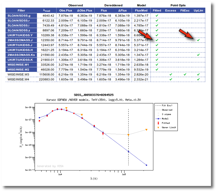
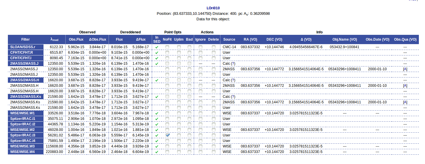
For instance, in this case (click in the image to enlarge):
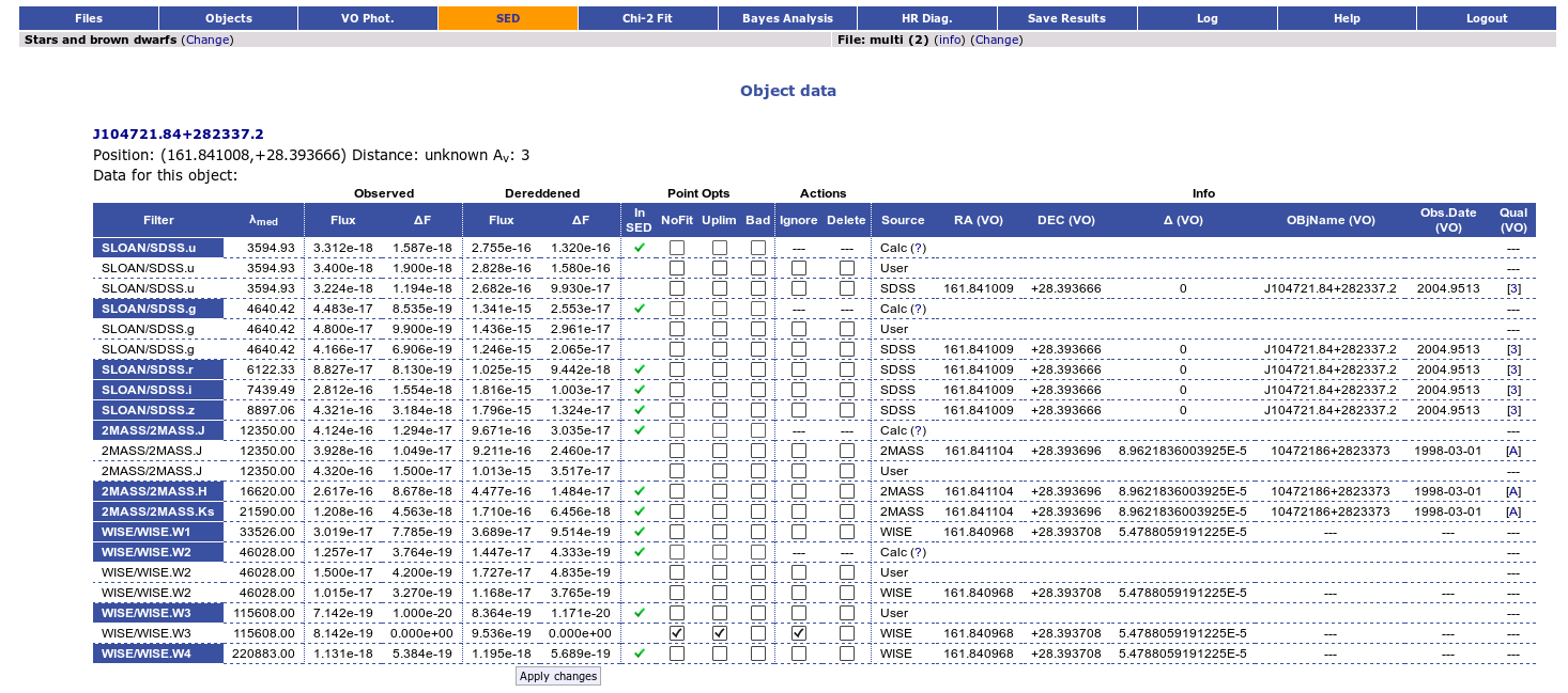
- For SLOAN/SDSS.u, 2MASS/2MASS.J and WISE/WISE.W2 there were two values for each filter, one from user input and one from a VO catalogue. VOSA has calculated an averate and it will be used in the final SED.
- For SLOAN/SDSS.g there are two values too. But, as one of them has been marked as 'nofit', the final average has been automatically marked as 'nofit' too.
- For WISE/WISE.W3 there are two values too. But the one coming from the WISE VO catalogue has been marked as ignore. Thus, this point is ignored and only the user value is there to be considered. VOSA does not need to calculate an average and the user value goes directly to the final SED.
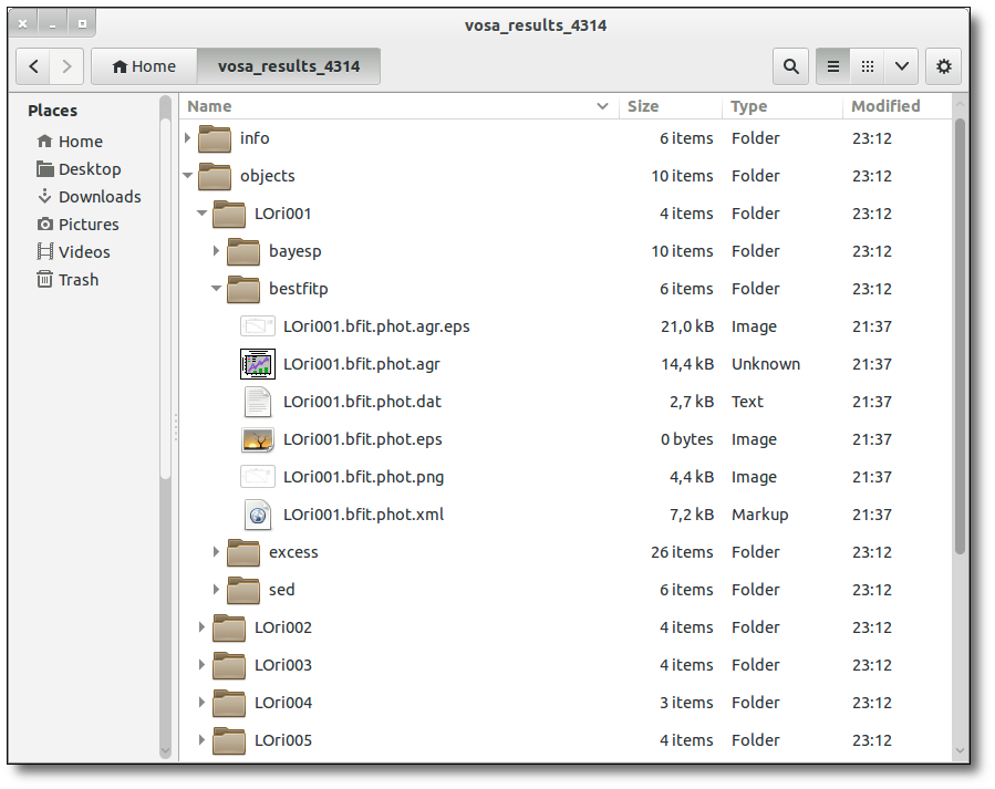
SED download
When you download the final resuls (see ) you will get a file (xml and/or ascii) with the final SED for each object. Most of the information is the same shown in the SED section of VOSA, but with some peculiarities.
When a data point has been calculated as an average of the photometry coming from different services (or user input file) some of the columns in the SED final file are built in terms of the original values for each catalogue. In particular:
- Δ (VO): this is the MAXIMUM value of all the Δ values for the data points combined to build this SED point.
- Δ_2 (VO): this is the MINIMUM value of all the Δ_2 values for the data points combined to build this SED point.
- Nobjs: this is the MAXIMUM value of all the Nobjs values for the data points combined to build this SED point.
- Qual (VO): if, for all the points combined to build this final SED point, the quality flag is the same, that value is shown here. Otherwise it is shown as 'mix'.
Excess
Most of the models used by VOSA for the analysis of the observed SEDs include only a photospheric contribution.
But the observed SED for some objects can include the contribution not only from the stellar photosphere but also from other components as disks or dust shells.
In these cases, some excess will appear and using the full SED for the analysis can be misleading.
Thus, VOSA offers the option to mark some part of the SED as "UV/Blue excess" or "Infrared excess" so that the corresponding points are not considered when the SED is analyzed using photospheric stellar models.
Infrared excess
VOSA tries to automatically detect possible infrared excesses.
Since most theoretical spectra used by VOSA correspond to stellar atmospheres only, for the calculation of the Χr2 in the 'model fit' the tool only considers those data points of the SED corresponding to bluer wavelengths than the one where the excess has been flagged.
(Some models, as the GRAMS ones, include other components as dust shells around the star. For those cases the points marked as 'infrared excess' will be also considered in the model fit).
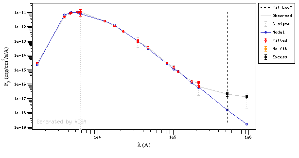
The last wavelength considered in the fitting process and the ratio between the total number of points belonging to the SED and those really used are displayed in the results tables.
The point where infrared excess starts is calculated, for each object, when you upload an input file, but it is also recalculated whenever the observed SED changes, that is:
- When VO photometry is added to the SED.
- When you delete a point in the SED or change something in the "SED" tab.
The excesses are detected by an algorithm based on calculating iteratively in the mid-infrared (adding a new data point from the SED at a time) the α parameter from Lada et al. (2006) (which becomes larger than -2.56 when the source presents an infrared excess). The actual algorithm used by VOSA is somewhat more sophisticated. A more detailed explanation is given below.
Apart from the automatic estimation made by VOSA, you can override this value specifying manually the point where infrared excess starts (so that more or less points are taken into account in the model fit) using the SED tab. Take into account that if you change the SED later (adding VO photometry or deleting a photometric point) this value will be recalculated again by VOSA.
It is also possible to specify the point where infrared excess start, for each object, as an 'object option' (10th column) in your input file. If you want to do this you have to include 'excfil:FilterName' (for instance: excfil:Spitzer/IRAC.I1) in the 10th column of the file. If you do that VOSA will not calculate the infrared excess for this object on upload and will accept the value given in the input file. But take into account that, if you change the SED later (adding VO photometry or deleting a photometric point) VOSA will recalculate the value even in this case.
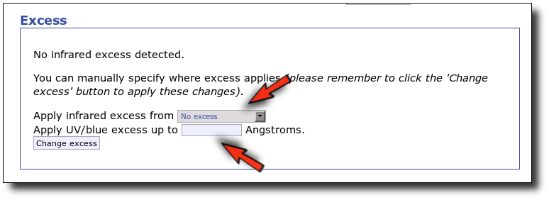
Finally, you also have the possibility of changing the point where infrared excess starts for all objects at the same time. In order to do that, go to the SED tab and look for the "excess" link in the left menu. Once there, you have a form where this can be done.
IR excess automatic detection algorithm
The algorithm used by VOSA to estimate the presence of infrared excess is an extension of the in the idea presented on Lada et al. (2006).The main idea is calculating, point by point in the infrared, the slope of the regression of the log-log curve showing $\nu F_{\nu}$ vs. $\nu$. At a first approximation, when this slope becomes smaller than 2.56, infrared excess starts.
In what follows, when we talk about regressions, we mean the regression of $y=log(\nu F_{\nu})$ as a function of $x=log(\nu)$, and taking into account observational errors as a weight for the regression. From error propagation, the "y" errors can be calculated as $\sigma(y) = \sigma(F_{\lambda})/(\ln10 F_{\lambda})$.
In order to avoid false detections due to "bad" photometric points, we refine the procedure as follows:
- We start at the first photometric point with $\lambda > 21500 A$.
- Points labeled as "nofit" are not considered in the algorithm.
- For each point (but the first one) we calculate:
- The linear regression of all the points from the first to this one (without taking into account those already labeled as "excess suspicious", see bellow).
- The $y$ value that would correspond to this point for a straight line starting on the first point and with slope=2.56. We call it $y_{\rm L}$.
- We mark the point as "excess suspicious" if it matches both of the following two criteria:
- The regression slope (b), plus the error in the slope, is smaller than 2.56, that is: $$b+\sigma(b) < 2.56 $$
- The observed value of $y$ is at least $3\sigma$ above the one predicted by the line with slope 2.56, that is: $$(y_{\rm obs} - y_{\rm L} ) > 3 \sigma(y)$$
- Points marked as "suspicious" will not be taken into account in further regressions.
- If two consecutive points are "suspicious" then VOSA marks the first of those points as the beginning of infrared excess.
- If one pointis suspcious and the next one isn't, then nothing happens. The first point (the suspicious one) will not be taken into account in further regressions, but we continue inspecting the next points.
- If the last point in the SED is suspicious, i.e., it matches both excess criteria, then that point is considered the beginning of inrrared excess even though the previous one did not match the criteria.
Apart from this, one more final criterium is applied. The slope (calculated as explained above) for at least one of the last two points in the SED must be sigma-compatible with being smaller than 2.56. $$b-\sigma(b) < 2.56$$
If this does not happen for any of the last two points, then there is no excess in the SED. The idea is that, if the infrared excess starts in some point it must continue for larger wavelengths. If that does not happen, any previous apparent detection of excess will be probably due to some "evil" combination of misleading points. In summary:
- The slope for at least one of the last two points in the sed must fulfill: $$b-\sigma(b) < 2.56$$
- two consecutive points must fulfill: $$b+\sigma(b) < 2.56 $$ $$(y_{\rm obs} - y_{\rm L} ) > 3 \sigma(y)$$ and then the infrared excess starts at the first of the two points.
- Or, if the last point in the SED meets those two criteria, even if the previous didn't, then the excess starts at the last point.
In the "Save Results", the user will be able to download files with a summary of the excess determination and with the details of each linear regression. These summary and details can also be visualized in the "SED" tab.
You can see some detailed examples of these calculations.
Fit refinement of the IR excess
When a model fit is completed, VOSA compares the observed SED with the best fit model synthetic photometry and makes a try to redefine the start of infrared excess as the point where the observed photometry starts being clearly above the model.
The procedure is as follows:
- If there is a point previously marked as the start of infrared excess VOSA starts the checking at that point.
- If not, VOSA starts in the medium point among those with λ > 21500A.
- For each point, VOSA checks for two criteria: $$\frac{F_{obs}-F_{mod}}{\Delta F_{obs}} > 3$$ $$\frac{F_{obs}-F_{mod}}{F_{mod}} > 0.2$$ that is, in plain words: the observation must be above the model, at least at a 3σ level, and the difference between both must be "significant".
- Both criteria must be fulfilled to consider that a point has excess (unless $\Delta F_{obs}=0$, that only the second crterium can be applied).
- If the criteria are fulfilled at the first point (thus, suspicious of 'fit excess') we check the previous point (smaller wavelength) and continue till one point doesn't match the criteria.
- If the criteria are NOT fulfilled at the first point (thus, no 'fit excess' detected) we check the next point (bigger wavelength) and continue till one point matches the criteria.
Let's see some examples.
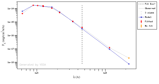
In the next case, when comparing the observed photometry with the model, VOSA sugests that the real infrared excess starts later than when the automatic algorith had detected:
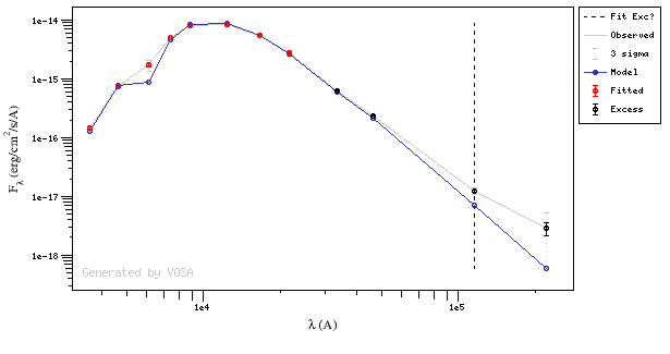
In this image, looking at the fit, there is no apparent infrared excess (although the automatic algorithm had detected it):
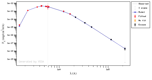
In the following case, according to the "fit excess" criteria there is no infrared excess. This is due to the big observational errors. Instead, the automatic algorithm had detected it:
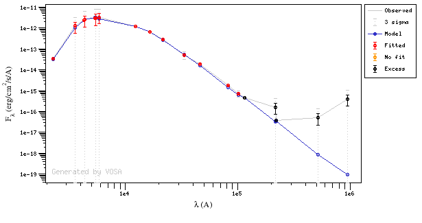
Onthe other hand, there are cases where the automatic detection algorith had not detected infrared excess but according to the fit, we see some excess:
And, obviously, in many cases both algorithms give the same result:
If for some objects the IR excess starting point calculated in this way is different from the one previosly calculated by the automatic algorithm, VOSA offers you the option to "Refine excess". If you click the corresponding button you will see the list of objects where this happens, the filters where excess starts according to both algorithms for each case, and the possibility of marking the start of infrared excess in the point flagged by the fit refinement instead of the one previously calculated by VOSA. If you choose to do this, and given that this would change the number of points actually used in the fit for those objects, the fit results are deleted and you have to restart the fit process. But, in what follows, the IR starting point will be the one suggested by the previous fit.
UV/blue excess
In some cases, there is also some excess in the bluer (UV) part of the SED.
VOSA does not detect this automatically, but you can specify it so that the application does not consider these points in the fits either.
The UV/blue excess can be set in two different ways:
- Including it in the input file as an 'object option' with the syntax Veil:VALUE, where VALUE is the value in Angstroms of the last wavelength where UV excess applies. For instance, if you include Veil:6000 in the 10th column of your input file for a given object, all the points with λ<=6000A will be marked as "Blue excess" and they will not considered in the fits.
- Specifying this value manually in the SED tab.
Finally, you also can specify the same UV/blue excess range for all objects at the same time. In order to do that, go to the SED tab and look for the "excess" link in the left menu. Once there, you have a form where this can be done.
This Blue excess, as it happens with the infrared one, will not be taken into account for models that include not photospheric components (as the GRAMS ones).
An example
We have an object where VOSA detects infrared excess starting at the Paranal/VISTA.J filter.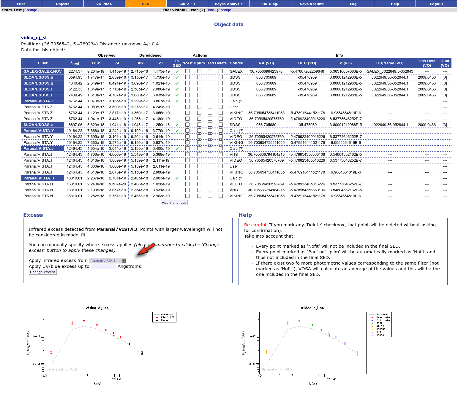
We are going to consider three different examples.
(1) Infrared excess only
First, we leave the excess as detected by VOSA, starting at VISTA.J.
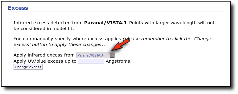
Those points are plotted in black in the SED.
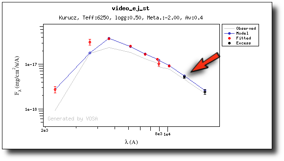
If we make a model fit for this object, the last two points in the SED won't be used. We see, in the results table, that only 8 of the 10 points have been used, and the wavelength of the last point fitted in the SED is the one for VISTA.J

And these two points are shown in black also in the fit plot.
(2) Both UV/blue and infrared excess
Now we decide to go back to the SED tab and we make a change:
- There is also some UV/blue excess up to 3000A (so that the GALEX.NUV point will not be considered for the fit either).
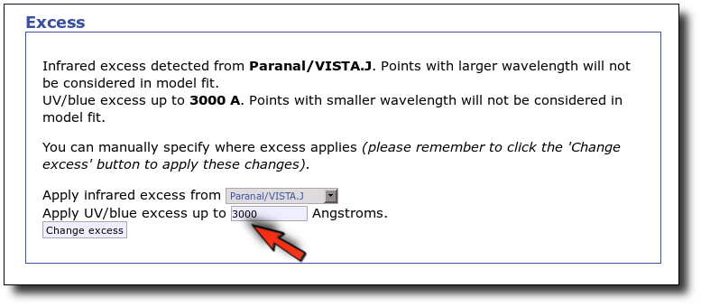
This changes the SED plot accordingly.
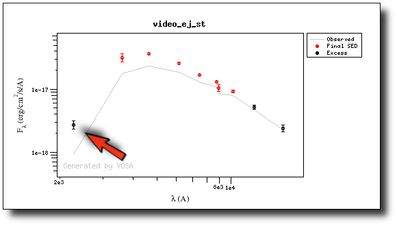
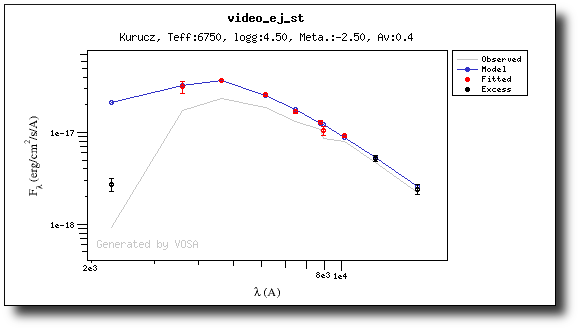
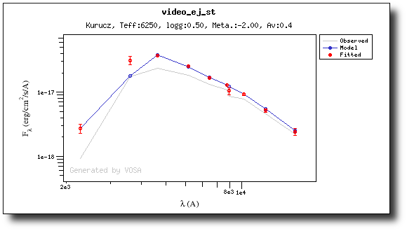
And when we repeat the model fit, the points that are fitted are only those that doesn't have excess now.
Actually, the best fit model is now a different one.

And the points in black in the fit plot are the ones corresponding to the excess that we specified manually (the GALEX.NUV point is not taken into account for the fit).
(3) No excess
As a last example, we go back to the SED tab and set that there is no infrared or UV/blue excess.
This changes the SED plot accordingly.
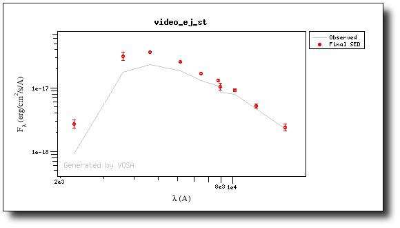
And when we repeat the model fit, all the points are considered for the fit now.

And all the points are shown in ref (fitted) in the plot.
Analysis
VOSA offers several options to analyze the observed Spectral Energy Distributions and estimate physical properties for the studied objects.
First, observed photometry is compared to synthetic photometry for different collections of theoretical models or observational templates in two different ways:
The Chi-square fit provides the best fit model and thus an estimation of the stellar parameters (temperature, gravity, metallicity, ...). It also estimates a bolometric luminosity using the distance to the object, the best fit model total flux and the observed photometry.
On the other hand, the Bayesian analysis provides the projected probability distribution functions (PDFs) for each parameter of the grid of synthetic spectra.
When these analysis tools are applied to observational templates (chi-square and bayes), we obtain an estimation of the Spectral Type too.
Once the best fit values for temperature and luminosity have been obtained, it is possible to build an HR diagram using isochrones and evolutionary tracks from VO services and making interpolations to estimate values of the age and mass for each object.
Model Fit
One of the main analysis options of this application is the Model fit.
Here the observed SED for each object is compared to the synthetic photometry for several theoretical models using a chi-square test. This gives an estimate of the physical properties of the given object.
If you provide a range for the visual extinction (AV), this fitting will also consider it as a fit parameter, as explained below.
Fit
When a fitting process is started you can choose among a list of theoretical spectra models available in the VO. Only those that are checked will be used for the fit.
In the next step the application uses the TSAP protocol (SSAP for theoretical spectra) for asking the model servers which parameters are available to perform a search. According to that, a form is built for each model so that you can choose the ranges of parameters that you want to use for the fit. Take into account that:
- The fitting process implies queries to VO services, data sent through the network, a lot of calculations (some done by the services themselves and some done by the application)... That means that it could take a long time to get the final results.
- Using more models and wider ranges of parameters will imply a longer time for the fitting (specially if your file contains many objects) so be ready for a long waiting time in the next step.
- In some cases, the whole range of parameters offered by the models are not right for your objects. For instance, if you know, for whatever physical reasons, that your objects have small temperatures, choose only small temperatures in the forms to optimize the process.
- The response time has roughly linear dependence on the number of objects in the file (twice number of objects means twice waiting time). Thus, you could prefer splitting your input file in different ones (according to physical properties, pertenence to a group or other reasons) better than doing all the work in an only data file.
- If you decide to fit the extinction too (giving a range for AV) this will also increase the fitting time. Take into account that 20 different values of AV are considered for each object/model combination. Although this won't imply a fitting time 20 times larger, it also enlarges the calculation time.
Once the fit has been finished, you can see a list with the best fit for each object and, optionally, a plot of these fits.
Besides that, for each particular object, you can also see a list with the best 5 fits for each model sorted by χ2. For each result you can see the corresponding SED and plot (with the "See" button) or use the "Best" button to mark a different result as the preferred best one. If you do that, this fit will be highlighted and it will be the one that will be shown in the "Best fit" table later.
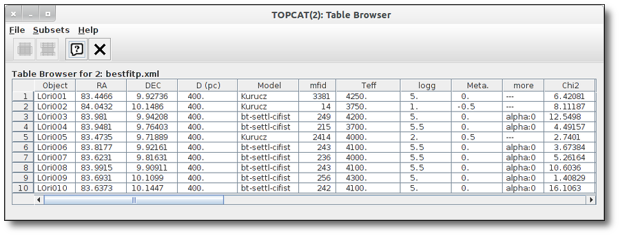
Best Fit
Once a fit has been done, you can see the Best Fit table with the best fit properties for each object.
A number of results are shown for each object:
- Object name, as given by the user.
- RA, Right Ascension as given by the user.
- DEC, Declination as given by the user.
- D(pc): distance in pc as given by the user (if the user does not provide a value, a typical default value of 10pc is used).
- Model name that best fits the data.
- Teff: effective temperature, in K, for the model that best fits the data.
- Log(G): logarithm of the gravity for the model that best fits the data.
- Metallicity: metallicity for the model that best fits the data.
- More: values for other (not so common) parameters used by the model.
- Χr2: value of the reduced chi-squared parameter for the fit (see below).
- Md: dilution factor. Value by which the model has to be multiplied to fit the data (see below).
- Ftot: Total flux (see below).
- ΔFtot: error for the total flux.
- Fobs/Ftot: fraction of the total flux obtained from the observed photometry (See below).
- Lbol/Lsun: Bolometric luminosity (See below).
- ΔLbol/Lsun: error for the Bolometric luminosity.
- λmax: value of the last wavelength considered for the fitting In order to avoid data with excess) (See below).
- AV: final value of AV used for dereddening the sed.
- ΔTeff: uncertainty for the effective temperature. It's estimated as half the grid step, around the given value, for this model.
- ΔLog(G): uncertainty for the logarithm of the gravity. It's estimated as half the grid step, around the given value, for this model.
- ΔMeta.: uncertainty for the metallicity. It's estimated as half the grid step, around the given value, for this model.
- ΔAV.: uncertainty in the value of AV (in the case that AV has been used as a fit parameter).
- R1. Estimate of the stellar radius obtained using Md and the distance (See below).
- ΔR1. Uncertainty on R1 (See below).
- R2. Estimate of the stellar radius obtained using logg and the distance (See below).
- ΔR2. Uncertainty on R2 (See below).
- M1. Estimate of the stellar Mass using Lbol and R1 (See below).
- ΔM1. Uncertainty on M1 (See below).
- M2. Estimate of the stellar Mass using Lbol and R2 (See below).
- ΔM2. Uncertainty on M2 (See below).
- Nfit/Ntot: Number of points considered in the fitting (not taking into account points with excess or points labeled as 'nofit') divided by the total number of observed points (See below).
- Link to a VOtable with the synthetic spectra corresponding to the best fit.
When the fit has been made with the option of calculating parameter uncertainties using a Monte Carlo method, a statistical distribution is obtained for these parameters and some other values are shown in this table:
- Teff,min,68, Teff,max,68: Minimum and maximum value for the effective temperature at the 68% confidence level. Calculated as the 14 and 84 percentiles of the distribution.
- Teff,min,96, Teff,max,96: Minimum and maximum value for the effective temperature at the 96% confidence level. Calculated as the 2 and 98 percentiles of the distribution.
- loggmin,68, loggmax,68: Minimum and maximum value for logg at the 68% confidence level. Calculated as the 14 and 84 percentiles of the distribution.
- loggmin,96, loggmax,96: Minimum and maximum value for logg at the 96% confidence level. Calculated as the 2 and 98 percentiles of the distribution.
- Metamin,68, Metamax,68: Minimum and maximum value for the Metallicity at the 68% confidence level. Calculated as the 14 and 84 percentiles of the distribution.
- Metamin,96, Metamax,96: Minimum and maximum value for the Metallicity at the 96% confidence level. Calculated as the 2 and 98 percentiles of the distribution.
- AV,min,68, AV,max,68: Minimum and maximum value for AV at the 68% confidence level. Calculated as the 14 and 84 percentiles of the distribution.
- AV,min,96, FV,max,96: Minimum and maximum value for AV at the 96% confidence level. Calculated as the 2 and 98 percentiles of the distribution.
- Ftot,min,68, Ftot,max,68: Minimum and maximum value for the total Flux at the 68% confidence level. Calculated as the 14 and 84 percentiles of the distribution.
- Ftot,min,96, Ftot,max,96: Minimum and maximum value for the total Flux at the 96% confidence level. Calculated as the 2 and 98 percentiles of the distribution.
Extinction fit
If a range for the visual extinction (AV) is given, it will also be considered a fit parameter.
You can provide this range for each object in two different ways:
- In the input file (10th column). See Upload file format section for more info.
- In the "Objects: extinction" tab.
If you don't provide a range for AV, the default value provided by you (also in the input file or the Extinction tab) will be used.
If you provide a range, like for instance AV:0.5/5.5, the fit service will compare each particular file of the model with the observed SED dereddened using 20 different values for AV in that range. Then the best fit models will be returned by the service with the best corresponding value of AV.
Reduced chi-square
The fit process minimizes the value of Χr2 defined as:
$$\chi_r^2=\frac{1}{N-n_p}\sum_{i=1}^N\left\{\frac{(Y_{i,o}-M_d Y_{i,m})^2}{\sigma_{i,o}^2}\right\}$$Where:
| N: | Number of photometric points. |
| np: | Number of fitted parameters for the model. (N-np are the degrees of freedom associated to the chi-square test) |
| Yo: | observed flux. |
| σo: | observational error in the flux. |
| Ym: | theoretical flux predicted by the model. |
| Md: | Multiplicative dilution factor, defined as: $M_d=(R/D)^2$, being R the object radius and D the distance between the object and the observer. It is calculated as a result of the fit too. |
Visual goodness of fit
Two extra parameters, Vgf and Vgfb are also calculated as estimates of what we call the visual goodness of fit.
The underlying idea is that, some times, the fit seems to be good for the human eye but has a large value of
chi2. One reason why this could happen is that there are some points with very small observational
flux errors. Thus, even if the model reproduces the observation apparently well, the deviation can
be much smaller than the reported observational error (increasing the value of chi2).
Given that it could happen that some observational errors could be understimated, we have defined these
two vgf and vgfb as two ways to estimate the goodness of fit avoiding these "too small" uncertainties.
The precise definition of these two quantities is as follows:
- Vgf: Modified reduced chi2, calculated by forcing that the observational errors are, at least, 2% of the observed flux. That is, in precise terms,
- ${\rm Vgf}^2=\frac{1}{N-n_p}\sum_{i=1}^N\left\{\frac{(Y_{i,o}-M_d Y_{i,m})^2}{a_{i,o}^2}\right\}, $
where- $\sigma_{i,o} \leq 0.02 Y_{i,o} \Rightarrow a_i = 0.02 Y_{i,o}$
- $\sigma_{i,o} \geq 0.02 Y_{i,o} \Rightarrow a_i = \sigma_{i,o}$
- ${\rm Vgf}^2=\frac{1}{N-n_p}\sum_{i=1}^N\left\{\frac{(Y_{i,o}-M_d Y_{i,m})^2}{a_{i,o}^2}\right\}, $
- Vgfb: Modified reduced chi2, calculated by forcing that the observational errors are, at least, 10% of the observed flux. That is, in precise terms,
- ${\rm Vgf_b}^2=\frac{1}{N-n_p}\sum_{i=1}^N\left\{\frac{(Y_{i,o}-M_d Y_{i,m})^2}{b_{i,o}^2}\right\}, $
where- $\sigma_{i,o} \leq 0.1 Y_{i,o} \Rightarrow b_i = 0.1 Y_{i,o}$
- $\sigma_{i,o} \geq 0.1 Y_{i,o} \Rightarrow b_i = \sigma_{i,o}$
- ${\rm Vgf_b}^2=\frac{1}{N-n_p}\sum_{i=1}^N\left\{\frac{(Y_{i,o}-M_d Y_{i,m})^2}{b_{i,o}^2}\right\}, $
These two parameters can help to estimate if the fit "looks good" (in the sense that the model is close to the observations). But, in any case, the best fit selected by VOSA will be the one with the smallest value of $\chi^2$.
Observational errors
The values of the observational errors are important because they are used to weight the importance of each photometric point when calculating the Χr2 final value for each model.
When σ=0 (that is, when there is not a value for the observational error) VOSA assumes that, in fact, the error for this point is big, not zero.
In practice, VOSA does as follows:
- Calculate the biggest relative error present in this SED. δ=Max(σi/Fluxi)
- Sum 0.1 to this maximum relative error: δ+0.1 = Max(σi/Fluxi) + 0.1
- Calculate the corresponding error: σi=(δ+0.1)*Fluxi
- This will be the value of σ used, during the fit, for any photometric point with a zero observational error.
- That is, these points will be the ones less important when making the fit
Excess
Since the theoretical spectra correspond to stellar atmospheres, for the calculation of the Χr2 the tool only considers those data points of the SED corresponding to wavelengths bluer than the one where the excess has been flagged.
The excesses are detected by an algorithm based on calculating iteratively in the mid-infrared (adding a new data point from the SED at a time) the α parameter from Lada et al. (2006) (which becomes larger than -2.56 when the source presents an infrared excess). See the Excess help for details about the algorithm.
The last wavelength considered in the fitting process and the ratio between the total number of points belonging to the SED and those really used are displayed in the results tables.
Excess fit refinement
When the fit has been done, VOSA compares the observed SED with the best fit model synthetic photometry and makes a try to redefine the start of infrared excess as the point where the observed photometry starts being clearly above the model. See the Excess help for more details.
If for some objects the IR excess starting point calculated in this way is different from the one previosly calculated by the automatic algorithm, VOSA offers you the option to "Refine excess". If you click the corresponding button you will see the list of objects where this happens, the filters where excess starts according to both algorithms for each case, and the possibility of marking the start of infrared excess in the point flagged by the fit refinement instead of the one previously calculated by VOSA. If you choose to do this, and given that this would change the number of points actually used in the fit for those objects, the fit results are deleted for these objects and the fit process is restarted for them (the results for other objects will remain unchanged). But, in what follows, the IR starting point will be the one suggested by the previous fit.
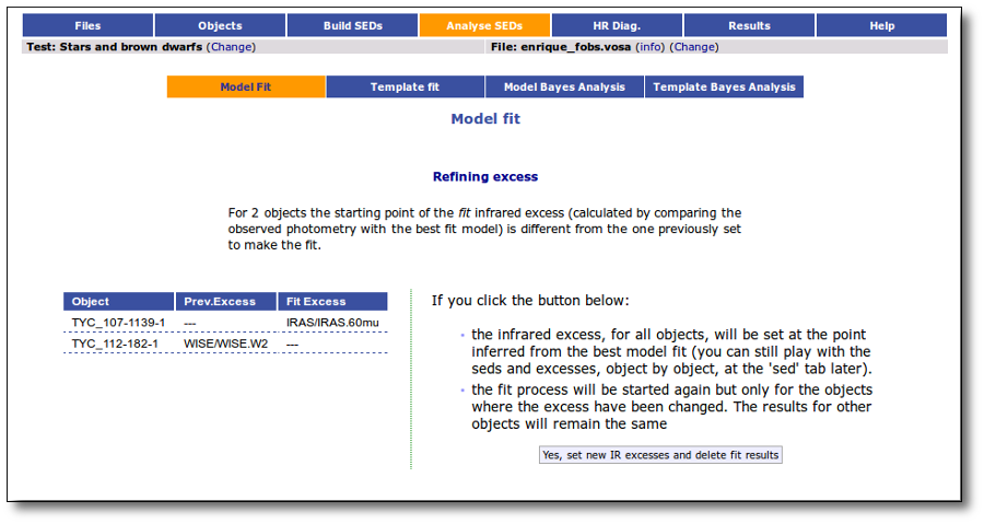
Synthetic photometry
Each theoretical spectra is a function Fi(λ) with units erg/cm2/s/Â.
Each filter is represented by a dimensionless response curve Gf(λ)
The synthetic photometry corresponding to the Fi spectra when it is observed through the filter Gf can be expressed as an integral: $$F_{i,f}=\int_{\lambda}F_i(\lambda) \ N_f(\lambda) \ d\lambda$$ where Nf(λ) is the normalized filter response function defined as: $$N_f(\lambda) = \frac{G_f(\lambda)}{\int G_f(x) \ dx}$$
Total flux and Bolometric luminosity
The best fitting model is used to infer the total observed flux for each source of the sample. We note that if the model reproduces the data correctly, this correction is much more accurate than the one obtained using a bolometric correction derived only from a color.
Total observed flux
The total theoretical flux for the object would be calculated as the integral of the whole model (multiplied by the corresponding Md factor): $$F_M = \int {\rm Md \cdot F_M}(\lambda) \ d\lambda$$
In order to estimate the total observed flux for the object, we want to substitute the fluxes corresponding to the observing filters by the observed ones, so that as much as the flux as possible comes from the observations. $${\rm Ftot} = \int{\rm Md \cdot F_M(\lambda) \ d\lambda} \ + {\rm Fobs} - {\rm Fmod} $$
The theoretical density flux corresponding to the observed one $\rm F_{o,f}$ can be calculated using the normalized filter transmision $N_f$: $$F_{M,f} = \int {\rm Md \cdot F_M}(\lambda) \cdot N_f(\lambda) \ d\lambda$$
In order to calculate the total observed flux, we have to estimate de amount of overlaping among diferent observations. In order to do that we, first, approximate the coverage of each filter using its effective width, then we identify spectral regions where there is a continues filter coverage an, for each of those regions, we define a "overlapping factor" as: $$ {\rm over}_r = \frac{\sum {\rm W}_i}{\rm (\lambda_{max,r} - \lambda_{min,r})}$$
using these overlapping factors we can estimate the degree of oversampling in each region by the fact that several observations are sampling the same range of the spectra. And we can approximate the total observed flux as: $$ {\rm Fobs} = \sum_f\frac{ {\rm F}_{o,f} \cdot {\rm W}_{eff,f}}{ {\rm Over_f}} $$
And the same for the corresponding contributions from the model: $$ {\rm Fmod} = \sum_f\frac{ {\rm F}_{M,f} \cdot {\rm W}_{eff,f}}{ {\rm Over_f}} $$
Thus, the total flux is given by: $${\rm F}_{\rm tot} = F_M + \sum_f\frac{ [ {\rm F}_{o,f} - {\rm F}_{M,f}] \cdot {\rm W}_{eff,f}}{ {\rm Over_f}} $$
where $F_{M,f}$ and $F_{o,f}$ are the model and observed flux densities corresponding to the filter $f$.
The corresponding error in the total flux is calculated as: $$ \Delta {\rm Fobs} = \sqrt{ \sum_f \left(\frac{ \Delta{\rm F}_{o,f} \cdot {\rm W}_{eff,f}}{ {\rm Over_f}}\right)^2 } $$
You can see a detailed example about this calculations.
Bolometric luminosity
The tool scales the total observed flux to the distance provided by the user and therefore estimates the bolometric luminosities of the sources in the sample (in those cases where the user has not provided a realistic value of the distance, a generic value of 10 parsecs is assumed): $$L(L_{\odot}) = 4\pi D^2 F_{obs}$$ $$\left(\frac{\Delta L}{L}\right)^2 = \left(\frac{\Delta F_{obs}}{F_{obs}}\right)^2 + 4 \left(\frac{\Delta D}{D}\right)^2 $$Estimate of parameter uncertainties
VOSA uses a grid of models to compare the observed photometry with the theoretical one. That means that only those values for the parameters (Teff, logg, metallicity...) that are already computed in the grid can be the result of the fit. For instance, if the grid is calculated for Teff=1000,2000,3000 K, the best fit temperature can be 2000K, but never 2250K (because there is not a 2250K model in the grid to be compared with the observations). But this only means that the model with 2000K, reproduces the observed SED better that the other models in the grid. And it could happen that, if it were in the grid, the model with 2200K were a better fit.
Thus, by default, VOSA estimates the error in the parameters as half the grid step, around the best fit value, for each parameter. For instance, if we obtain a best fit temperature Teff=3750K for the Kurucz model, and given that the Kurucz grid is calculated at 3500,3750,4000...K, the grid step around 3750 is 250K and the estimated error in Teff will be 125K.
Statistical approach
In order to obtain parameter uncertainties with a more statistical meaning, VOSA offers the option to "Estimate fit parameter uncertainties using an estatistical approach". If you mark this option the fit process will be different.
Taking the observed SED as the starting point, VOSA generates 100 virtual SEDs introducing a gaussian random noise for each point (proportional to the observational error). In the case that a point is marked as "upper limit" a random flux will be generated between 0 and ${\rm F}_{uplim}$ following a uniform random distribution.
VOSA obtains the best fit for the 100 virtual SEDs with noise and makes the statistics for the distribution of the obtained values for each parameter. The standard deviation for this distribution will be reported as the uncertainty for the parameter if its value is larger that half the grid step for this parameter. Otherwise, half the grid step will be reported as the uncertainty.
Although this means making 101 fit calculations for each object (instead of only one) the process time is not multiplied by 101. It takes only a little longer (around twice).
Estimate of stellar radius and mass
We can use the value of Md and the distance $D$ to estimate the stellar radius: $$M_d = \left(\frac{R}{D}\right)^2 $$ $$R_1 \equiv \sqrt{D^2 M_d} $$ $$\Delta R_1 = R_1 \frac{Δ D}{D} $$
But we can estimate the radius also using $T_{eff}$ and $L_{bol}$. $$L_{bol} = 4\pi\sigma_{SB} R^2 T_{eff}^4$$ $$R_2 = \sqrt{L_{bol}/(4\pi\sigma_{SB} T_{eff}^4)}$$ $$\Delta R_2 = R_2 \sqrt{\frac{1}{4} \left(\frac{\Delta L_{bol}}{L_{bol}}\right)^2 + 4 \left(\frac{\Delta T_{eff}}{T_{eff}}\right)^2}$$
We can estimate also the mass using $logg$ and $R$ $$ g = \frac{G_{Nw}M}{R^2} $$ $$ M = 10^{logg} R^2 / G_{Nw} $$
In this formula we can use either $R_1$ or $R_2$ to obtain two different estimate of the mass: $$ M_1 = 10^{logg} R_1^2 / G_{Nw} $$ $$\Delta M_1 = M_1 \sqrt{\ln(10)^2 (\Delta logg)^2 + 4 \left(\frac{\Delta R_1}{R_1}\right)^2} $$ $$ M_2 = 10^{logg} R_2^2 / G_{Nw} $$ $$\Delta M_2 = M_2 \sqrt{\ln(10)^2 (\Delta logg)^2 + 4 \left(\frac{\Delta R_2}{R_2}\right)^2} $$
WARNINGS.
Take into account that the values obtained, both for the mass and radius, will be make sense only if the value for the Distance is realistic. What's more, these values will be more trustable when Fobs/Ftot is closer to 1. Otherwise, the obtained values could not be realistic.
In the other hand, given that the uncertainty of $logg$ given by models is typically large, and SED analysis is not very sensible to the value of logg, take into account that the value of the Mass obtained using logg could be far from real.
Parameter polynomial fit
When you go to see all the fits for a particular object you will also see a section named "Parameter polynomial fit".
For each fit parameter, VOSA will take into account all the values obtained in the best fits and try to adjust a 2 degree polynomial to the (param,chi2) points.
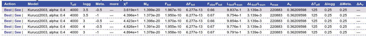
If this polynomial has a minimum and this minimum is in the range between the minimum and maximum values obtained for this parameter, VOSA will offer this value as possible "best fit value" for this parameter, trying to go further than the constraints due to the discrete nature of the model grid.
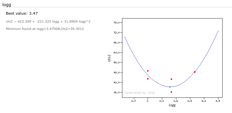
In some cases a mimimum is found but this is out of the range given by the obtained parameter values in the fit. In this case VOSA does not recommend the use of this value.
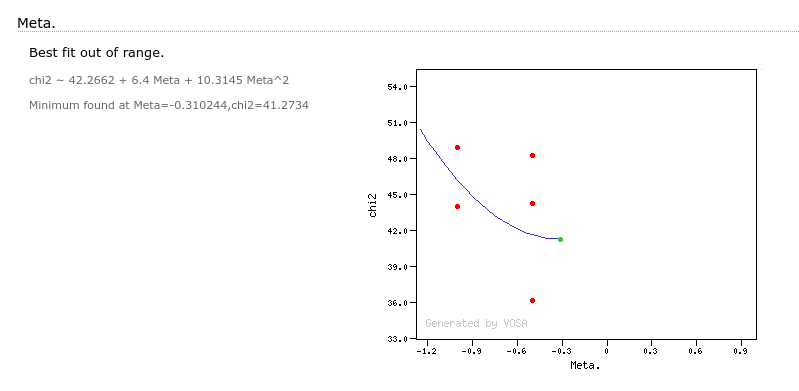
It can also happen that the parabola fit does not have a minimim but a maximum. Of course, the value of the parameter at the maximum does not provide better information.
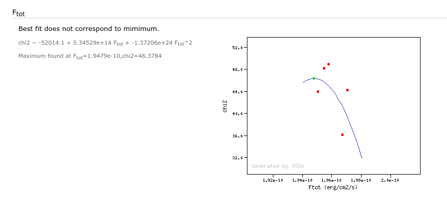
Partial refit
After you have finished the fit process, sometimes it is useful to make small changes in the SED for some objects and repeat the fit. But, when your file contains many objects it is boring and slow to repeat the fit process for all the objects when only a few SEDs have changed.
VOSA keeps track of what SEDs have been changed in a significant way after the fit, so that the current fit results could be not valid for those objects anymore (for instance, you edit the SED, add/remove some point, search for VO photometry, add VO photometry, change where the excess starts, change the value of extinction, etc.)
When you go back to the chi2 fit tab, VOSA will show you a message saying the the SED for some objects has been changed after the fit was finished and offers you the option of repeating the fit only for those objects. If you click in the "Repeat the fit process" button, the fit process will be done again with the same previous options (model choice, parameter ranges choices, etc) but only for the objects that have changed. The fit results for the other objects will remain the same.
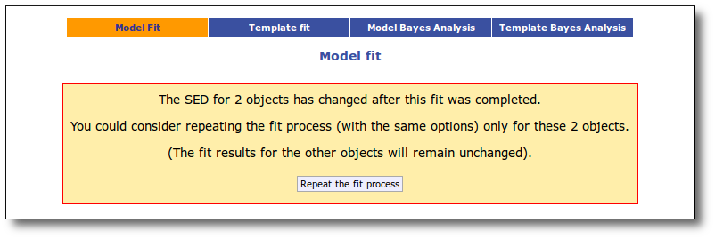
A particular case is the one when you choose to refine the excess setting the start of the IR excess at the point suggested by the model fit. When you do this, the fit is repeated only for the objects where the excess have changed (the results for other objects will remain unchanged).
Example
When we access the Chi-2: Model Fit tab we see a form with the available theoretical models, so that we can choose what ones we want to use in the fit. In this case we decide to try Kurucz and BT-Settl-CIFIST models. Thus, we mark them and click in the "Next: Select model params" button.
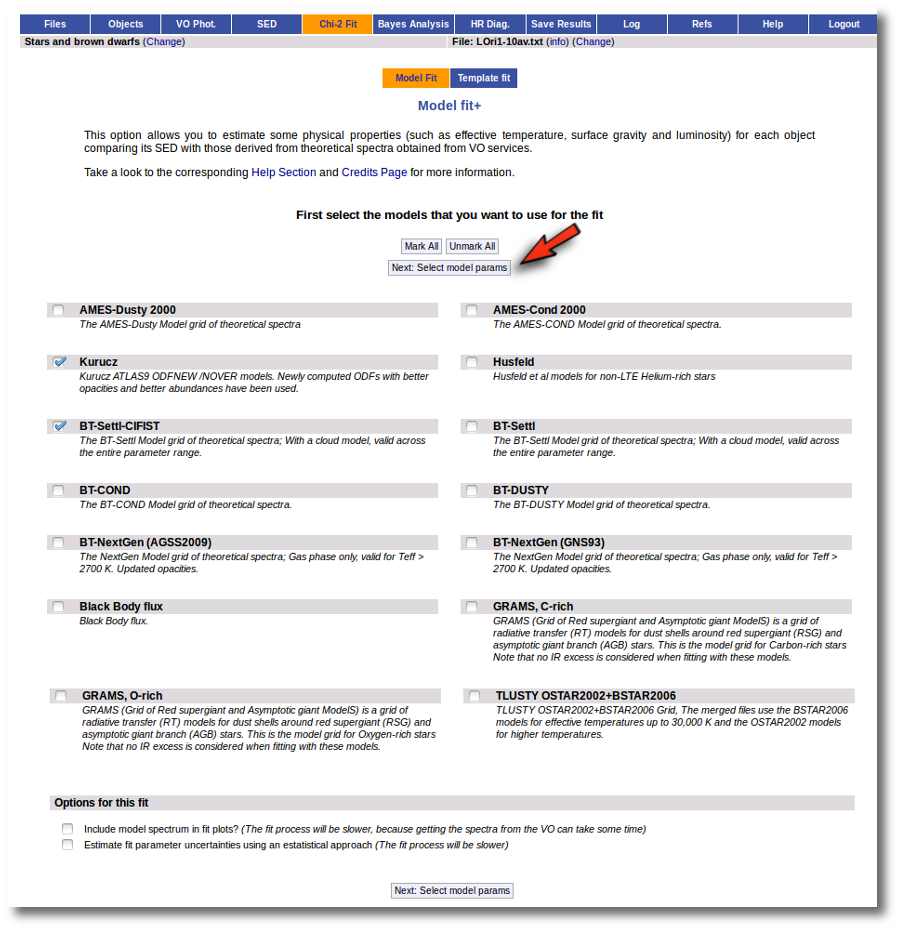
For each of the models, we see a form with the parameters for each model and the available range of values for each of them. We choose the ranges that best fit our case and then click the "Next: Make the fit" button.
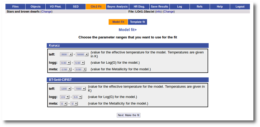
The fit process is performed asynchronously so that you don't need to stay in front of the computer waiting for the results. You can close your browser and come back later. If the fit is not finished, VOSA will give you some estimate of the status of the operation and the remaining time.
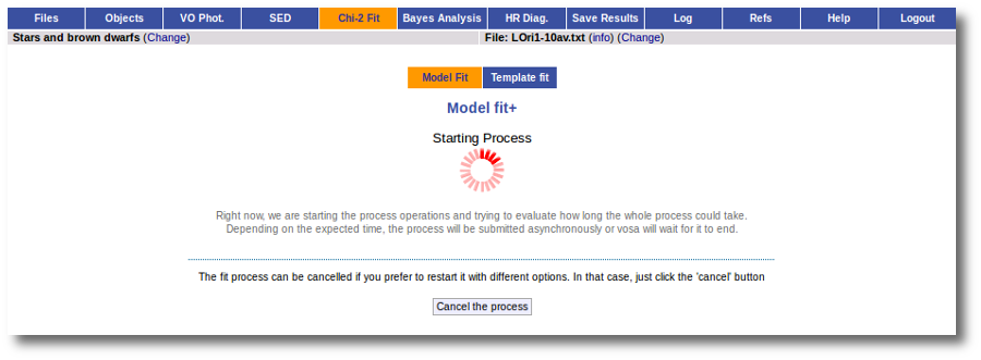
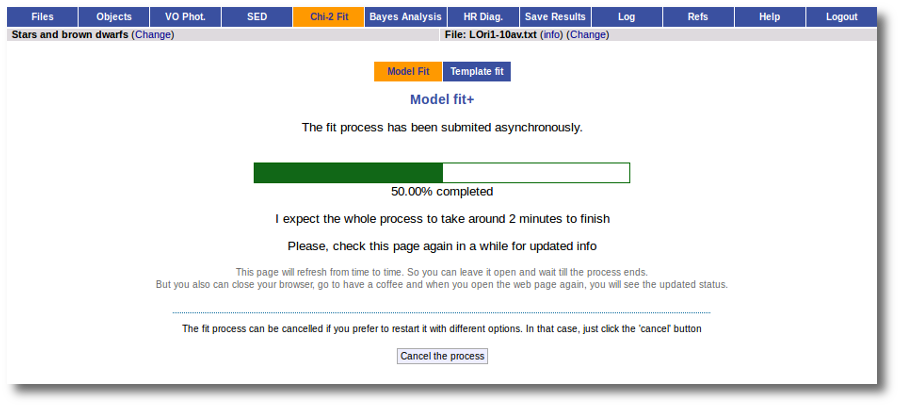
When the process finishes VOSA shows a list with the best fit model (that is, the one with a smaller value for the reduced chi-2) for each object. Optionally you can also see the best fit plots, with the observed SED and the corresponding synthetic photometry for the best fit model.
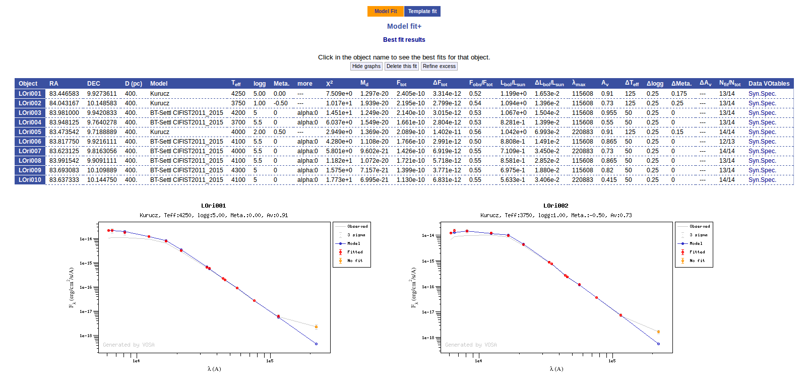
If we click in the LOri002 object name in the table we can see the 5 best fits for each collection of models. And clicking on the "See" link on the right of each fit, we can see the details about it.
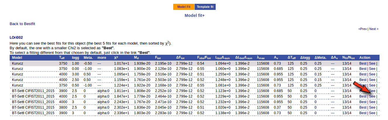
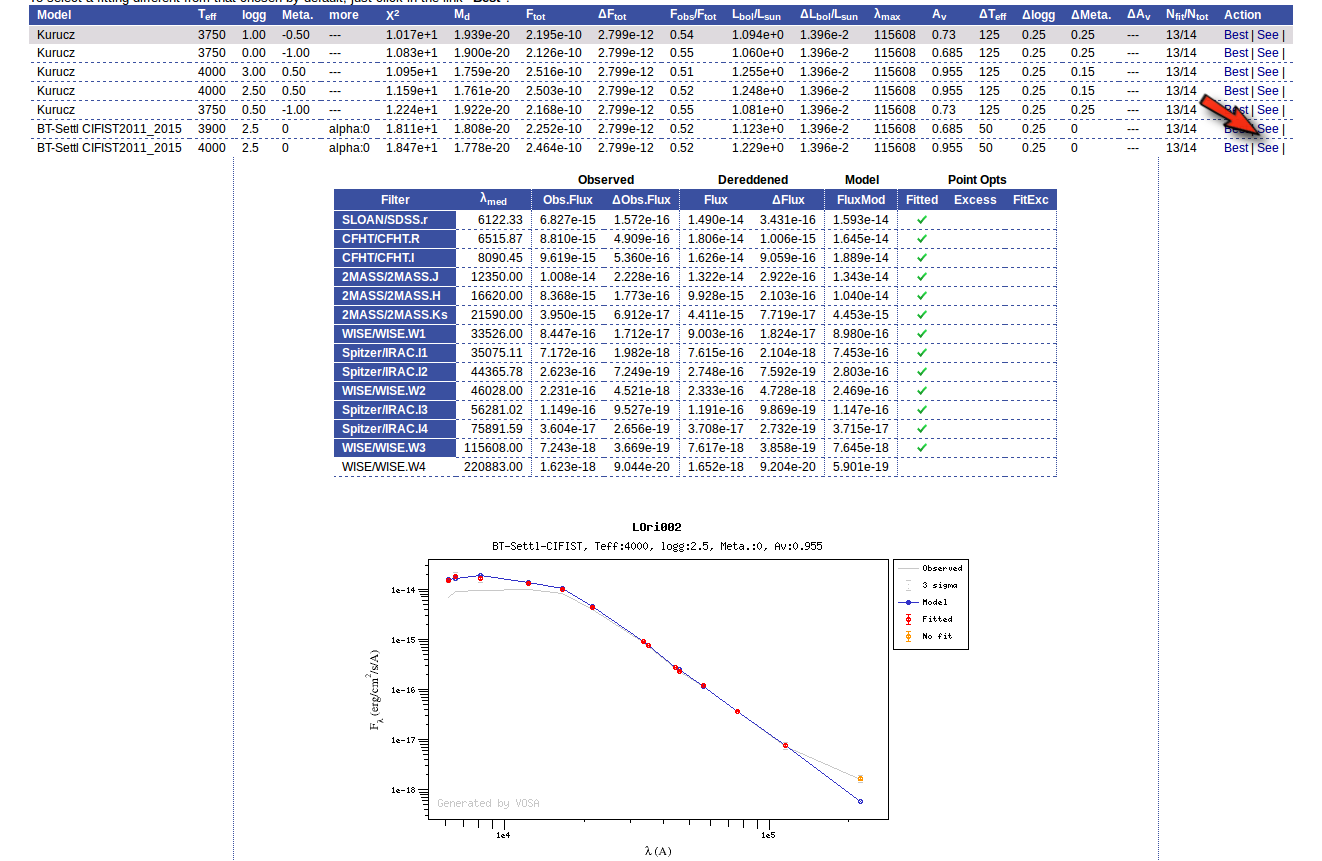
Sometimes the fit with the best Χ2 is not the one that the user considers the best one, maybe for physical reasons, taking into account the obtained values of the parameters, or maybe because one prefers a model that fits better some of the points even having a larger Χ2... Whatever the reason, we have the option to mark as Best the model that we prefer. In order to do that we just click in the Best link at the right of the fit that we prefer. In this case, just as an example, we choose the second BT-Settl one for LOri002.
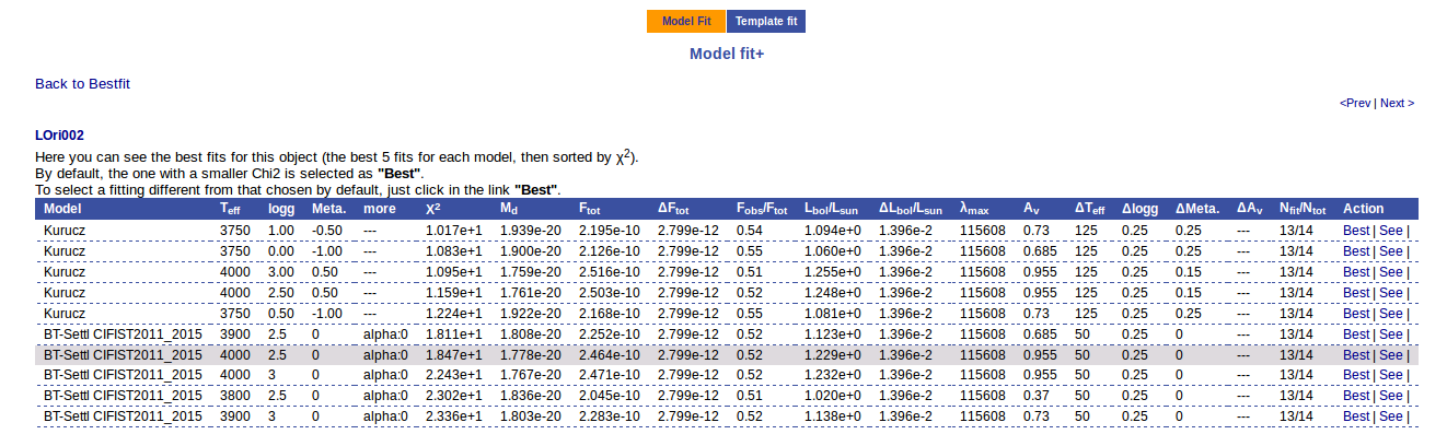
And, when we go back to the best fit list, we see that the one for LOri002 has changed.
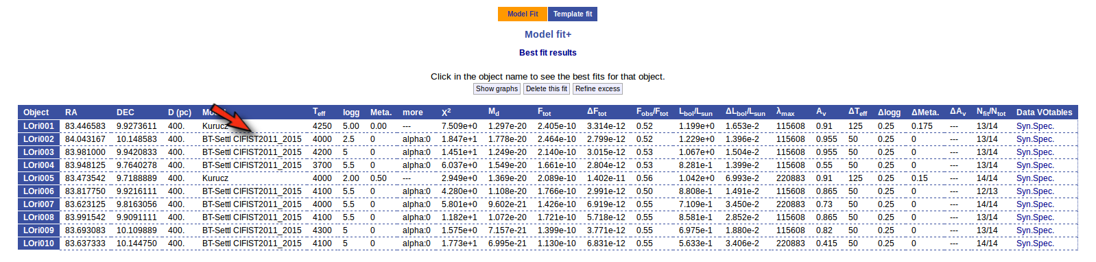
For some objects, for instance LOri10, we see a vertical dashed line in the plot at the point where the observed fluxes start being clearly above the model ones. VOSA marks it this way so that you are aware that infrared excess could start here.
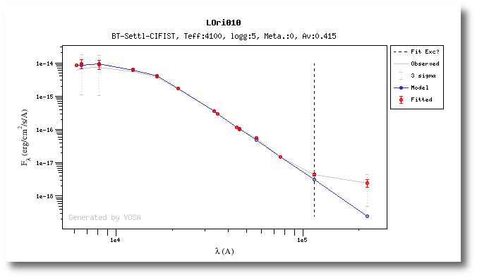
If we click in the "Refine excess" button, we can see the list of objects where VOSA detects a possible infrared excess starting at a point different from the one previously detected.
If we click the "Yes, set new IR excesses and delete fit results" button, the start of infrared excess will be flagged at the point coming from the fit comparison and these fit results will be deleted. Then we could restart the fit taking into account the new infrared excesses.
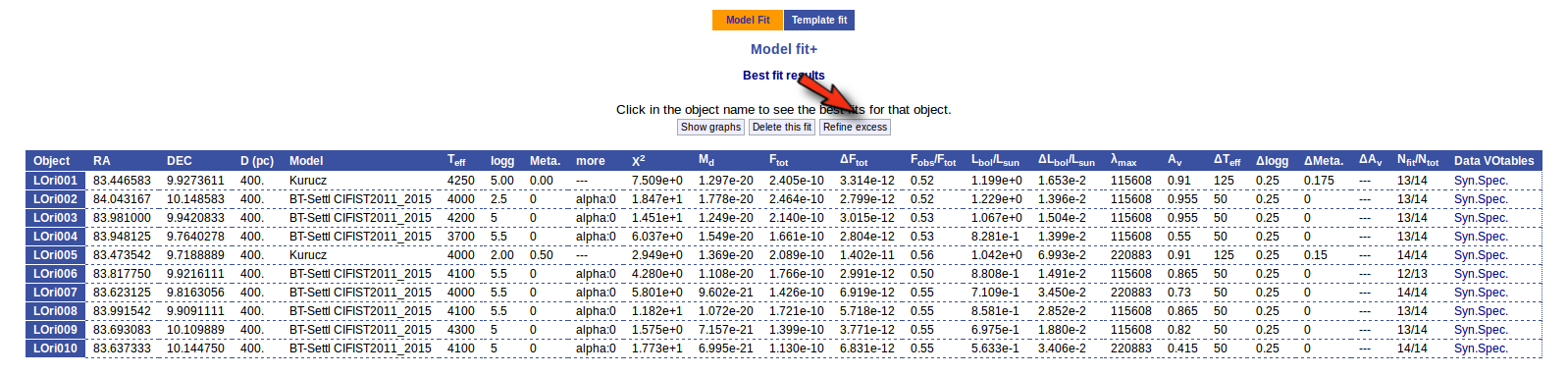
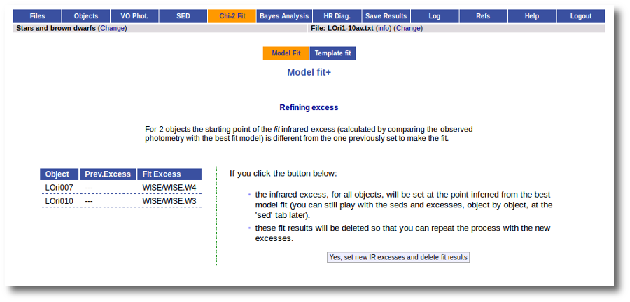
We also have the option of deleting these fit results so that we can restart the process with different options. And we do so clicking in the "Delete" button.
VOSA asks us for confirmation, we confirm the decision, and we see the initial form again.
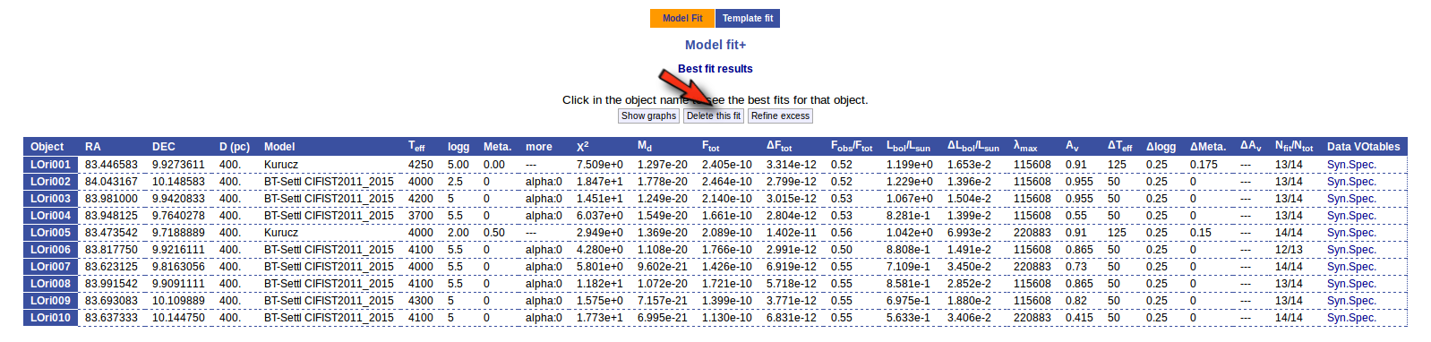
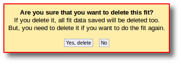
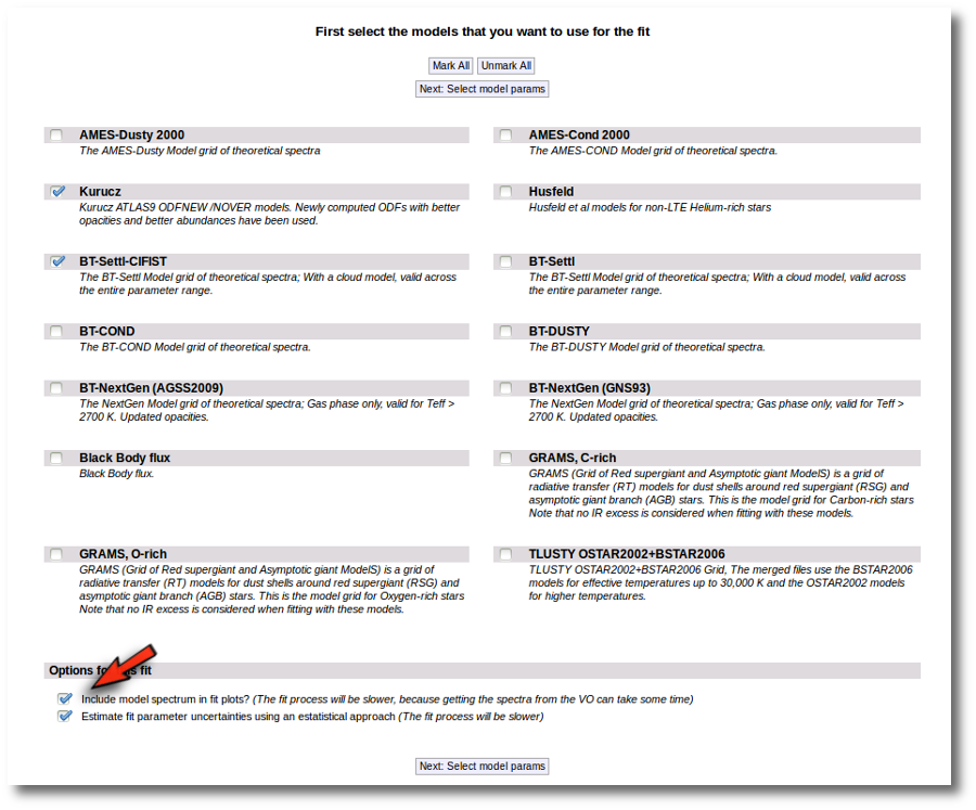
We select the same models again but we also mark the two extra options at the bottom.
When the fit process ends, we see two main differences in the results:
- The values of the estimated errors for the parameters are now different:
- The model spectrum is included in the fit plots.
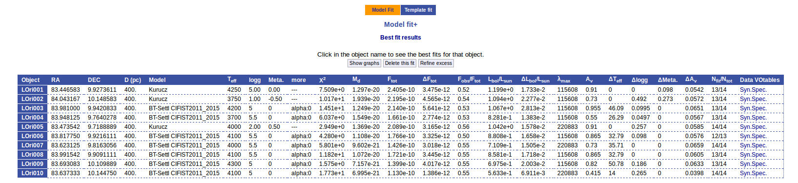
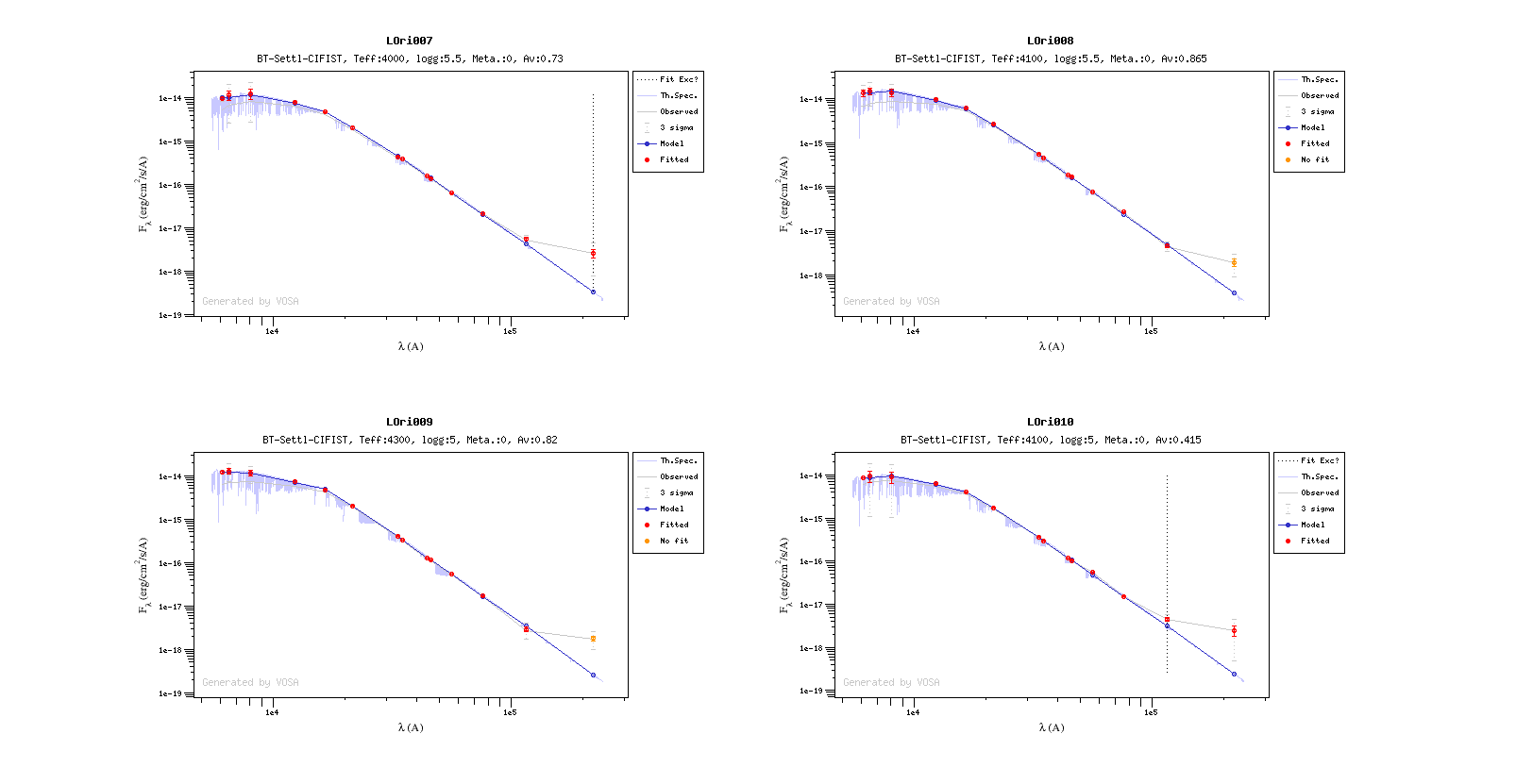
Bayes analysis
While the chi-square fit gives the best fit model for each object, the Bayesian analysis provides the projected probability distribution functions (PDFs) for each parameter of the grid of synthetic spectra.
The procedure followed by VOSA to perform a Bayesian analysis of the model fit is as follows:
- We first calculate a $\chi^2$ model fit as explained in [Model fit] .
- Then we assign a relative probability for each model as: $$W_i = \exp(-\chi_i^2/2)$$
- Using this, the probability corresponding to a given parameter value $\alpha_j$ is given by:
$$P(\alpha_j) = \sum_i W_i$$
where the sum is performed over all the models with that value for that parameter.
- We finally normalize these probabilities, for each parameter, dividing by the total probability (the sum of the probilities obtained for each value). $$P'(\alpha_j) = \frac{P(\alpha_j)}{\sum_i P(\alpha_i)}$$
In the case that you have decided to consider Av as a fit parameter (giving a range of Av values to try), the probability distribution for Av is calculated too.
Example
We enter the "Model Bayes Analysis" tab and we see a form with the available theoretical models, so that we can choose what ones we want to use in the fit. In this case we decide to try Kurucz and BT-Settl-CIFIST models. Thus, we mark them and click in the "Next: Select model params" button.
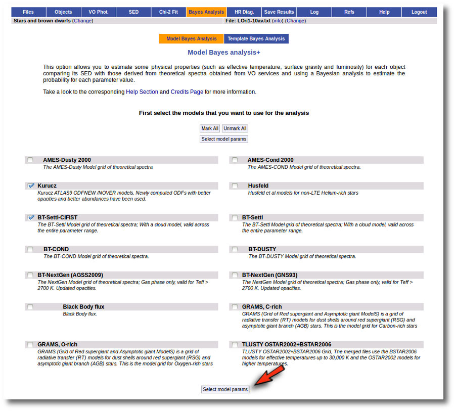
For each of the models, we see a form with the parameters for each model and the available range of values for each of them. In this case we are going to try the full range of parameters, so we leave the form as it is and then click the "Next: Make the fit" button.
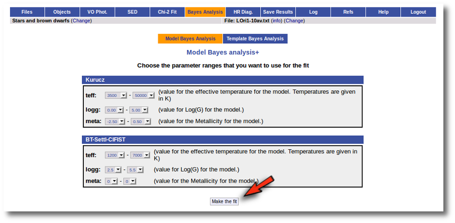
In this case, VOSA will have to calculate the chi-square fits and then use them to perform the analysis. The fit and analysis process is performed asynchronously so that you don't need to stay in front of the computer waiting for the search results. You can close your browser and come back later. If the process is not finished, VOSA will give you some estimation of the status of the operation and the remaining time.
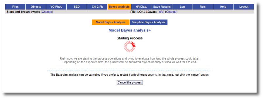
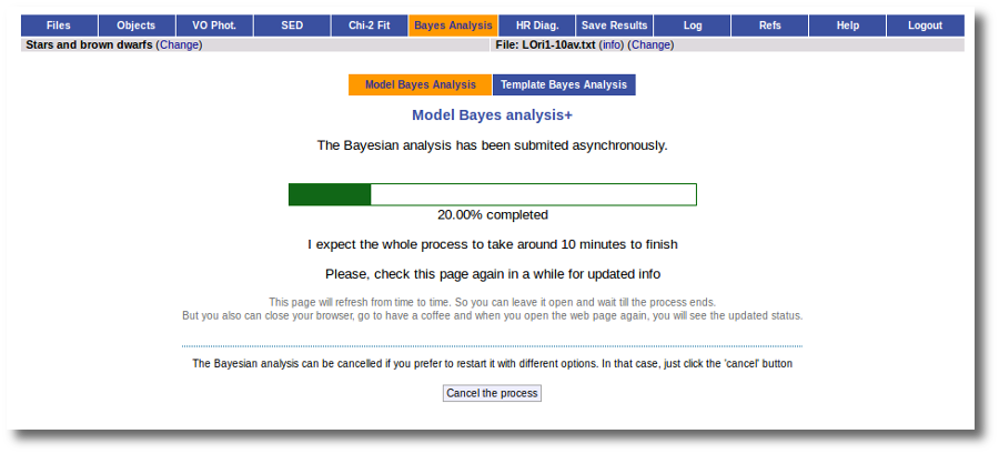
When the process finishes VOSA shows us a list with, for each object and each model collection, the most probable value for each parameter and its probability.
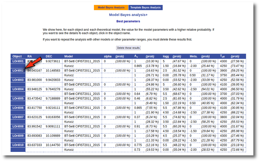
And if we click in one of the object names, we can see all the details of the analysis for this object.
We see first the probability of each value of each model parameter (only those values with a non-negligible probability are shown).
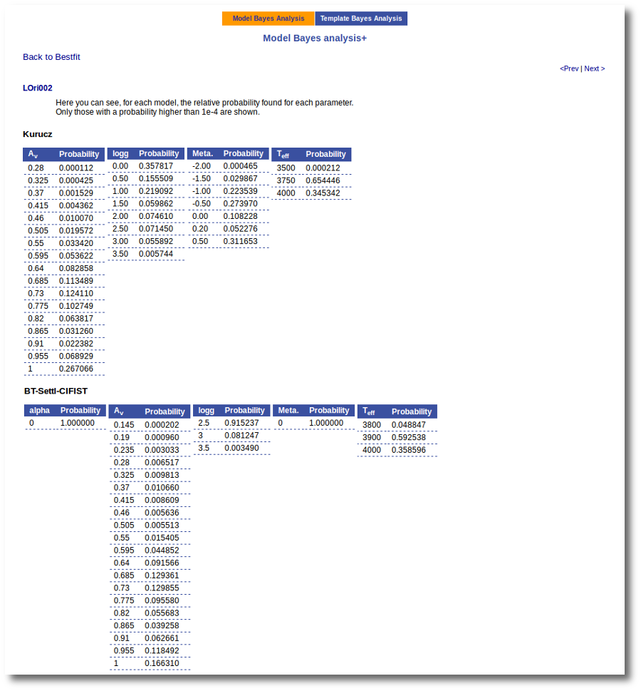
And then some simple plots of these probability distributions.
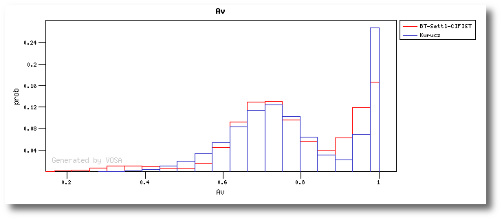
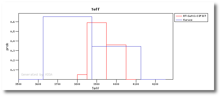
Template Fit
In some occasions, the limited understanding of the physical processes and/or the nature of some astronomical objects makes the theoretical models failed to reproduce with good accuracy the real observations. In this case, the comparison with benchmark objects, whose properties can be accurately determined without the use of models are largely preferred.
VOSA offers the possibility of performing both the Χ2 fitting and Bayes Analysis with standard objects. Four template collections covering M, L and T spectral types are now available: Chiu et al. (2006); Golimowski et al. (2004); Knapp et al. (2004); Kirkpatrick et al. (1991, 1999), McLean & Kirkpatrick7 and the SpeX Library. Take a look to the corresponding Credits Page for more information about these collections.
Take into account that these templates are usually the observed espectra of some well known objects and that means that the wavelength coverage of these spectra is not as wide as it is for most theoretical models. This implies that it is not possible to calculate the photometric photometry for all the filters, but only for the ones that are fully covered by the observed spectrum. In practice this means that only a few of the points in the observed SED will be used when comparing with templates. Thus, in some cases you will receive a "Not enough points to make a fit" message (even having quite many points in the SED). In any case, the number of points used for the fit will be shown in the results table and you can see which points have been actually fitted in the plots.
This is the main reason why, for template fitting, the AV extinction parameter is NOT considered a fit parameter. Having extra parameters would imply that less objects could be fitted. The value for AV given in the input file (or specified in the objects:extinction tab) will be used.
An example
We enter the Chi-2 Fit tab and then select the 'Template Fit' option. In this case we select all template collections and mark the 'include spectrum in plots' option to get nicer plots (the template spectra are not as big as theoretical spectra usually are, so using this option doesn't make the fit process much slower).
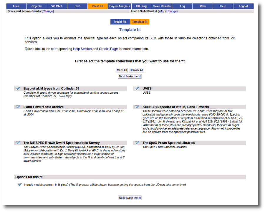
The fit process is performed asynchronously so that you don't need to stay in front of the computer waiting for th results. You can close your browser and come back later. If the fit is not finished, VOSA will give you some estimation of the status of the operation and the remaining time.
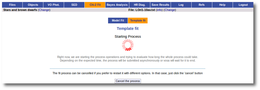
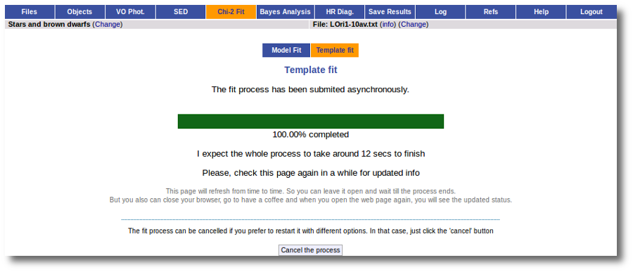
When the process finishes you can see a best fit results table with the spectral type that best fits the observed SED and, optionally, the corresponding plots.
In the plots you can see that only a few points in the SED are used for the fit (only 3 points for the Chiu et al. collection).
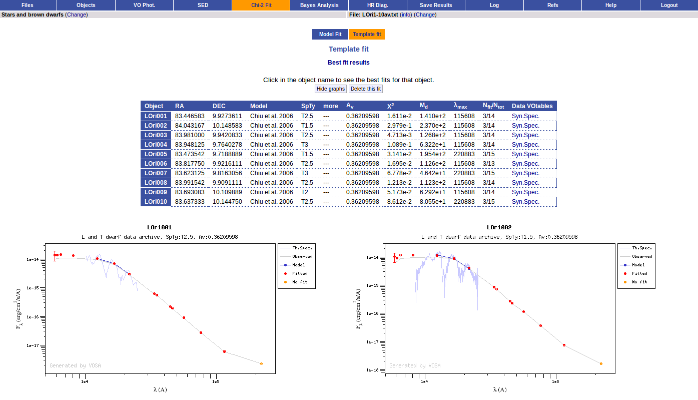
If you click in one of the object names you can see the best 5 fits for each collection. If you click in the "See" link you can see the corresponding plot. As you see, for the Spex Prism collection, we are able to fit 4 points (instead of the 3 ones that are fitted with the Chiu et al. one).
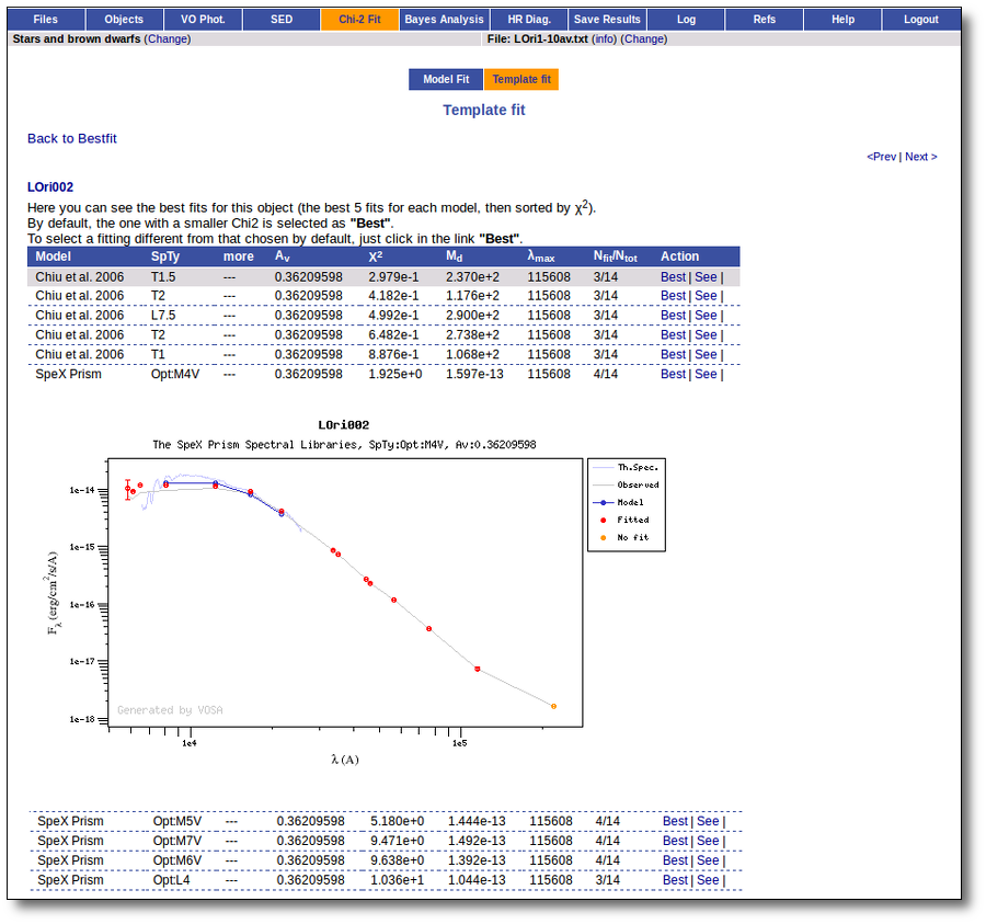
You have the option of choosing one of these fits as the best one if you wish, just clicking in the "Best" link on its right.
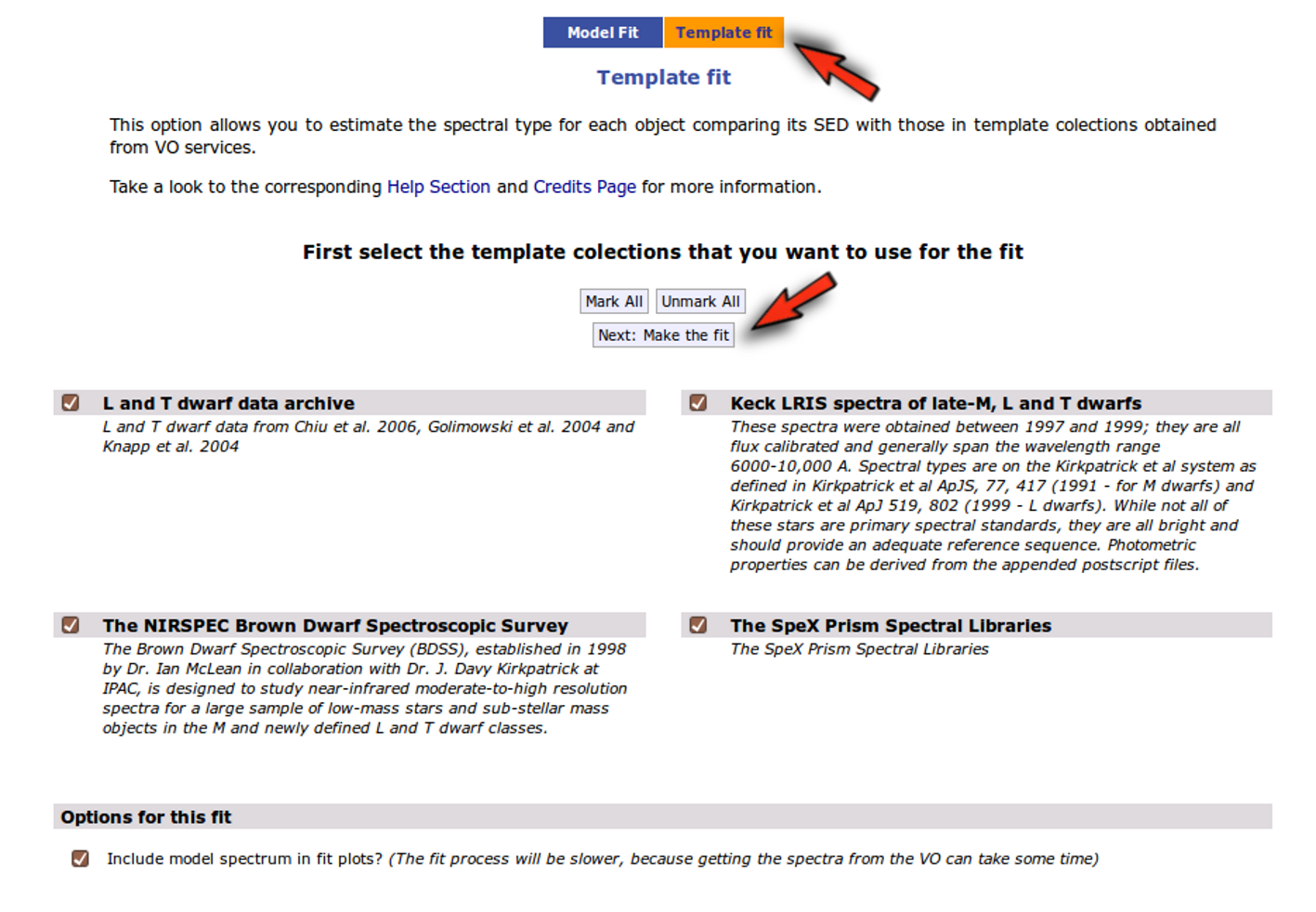
We see that only a few of the points in the SED are used for the fit. And in some cases there are not enough points.
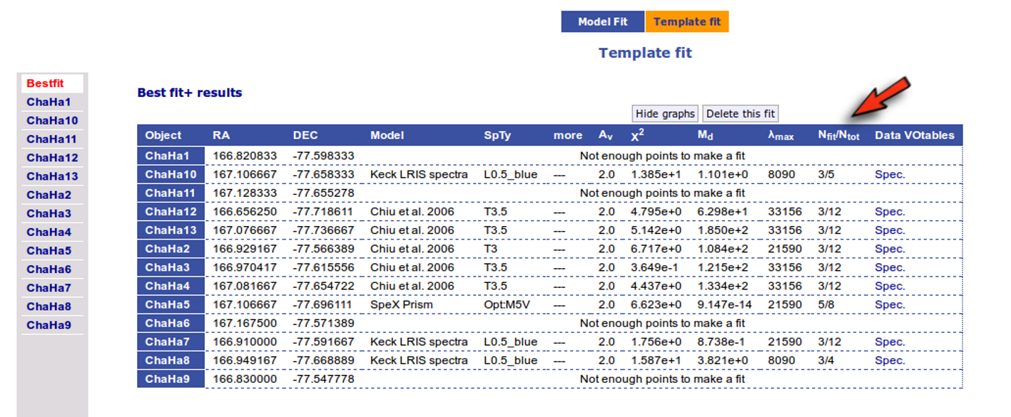

Bayes analysis
We can also make the bayes analysis using templates to get an estimation of the probability for each spectral type. Note that the probability for the AV value will always be 100% (because it's not actually fitted).
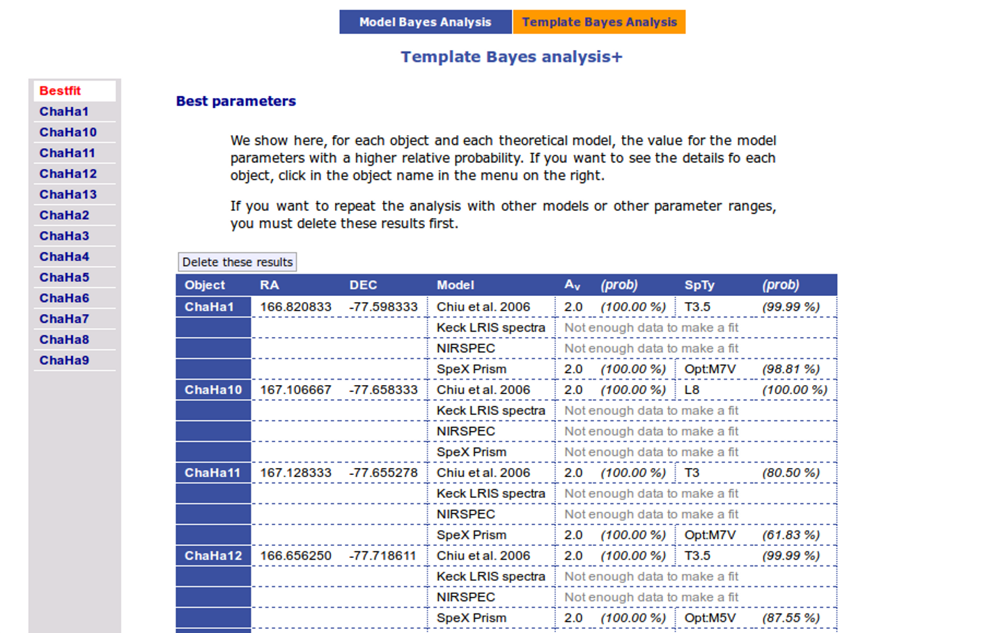
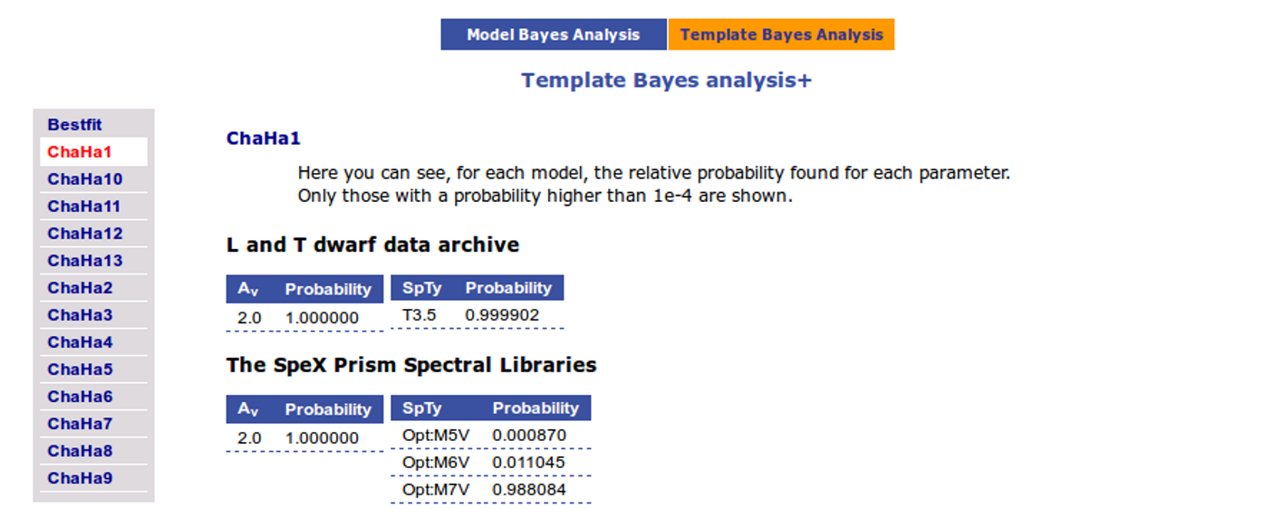
Template Bayesian analysis
We can also make the bayes analysis using templates to get an estimation of the probability for each spectral type.
Take into account that, as it happened in the Template fit, the AV extinction parameter is NOT considered a fit parameter.
For more details about the Bayesian approach, please read the section about Bayes analysis.
Example
We enter the "Template Bayes Analysis" tab and we see a form with the available template collections, so that we can choose what ones we want to use for the analysis. In this case we decide to try all of them and click in the "Make the fit" button.
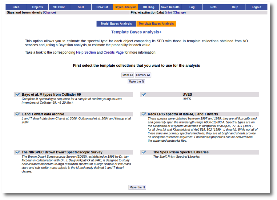
The fit and analysis process is performed asynchronously so that you don't need to stay in front of the computer waiting for the search results. You can close your browser and come back later. If the process is not finished, VOSA will give you some estimation of the status of the operation and the remaining time.
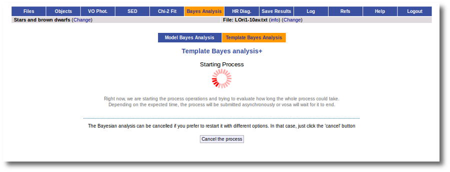
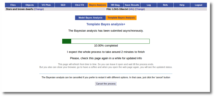
When the process finishes we can see the list of objects and the spectral type with the biggest probability for those collection where there were enough points to make the analysis.
Remember that Av is not considered a fit parameter for the analysis, so its value is fixed and its probability is always 100%.
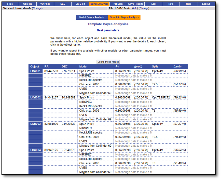
If we click in one object name, for instance, LOri001, we can see the probability of all the spectral types for each collection.
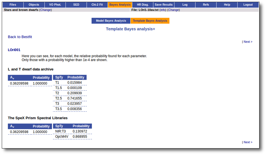
Binary Fit
The idea of "binary fit" appears when we face the case where an observed SED cannot be fitted well with a single theoretical model (that is, the flux comming from a single object) but it seems that it could be fitted well adding a second model (the flux comming from a second object).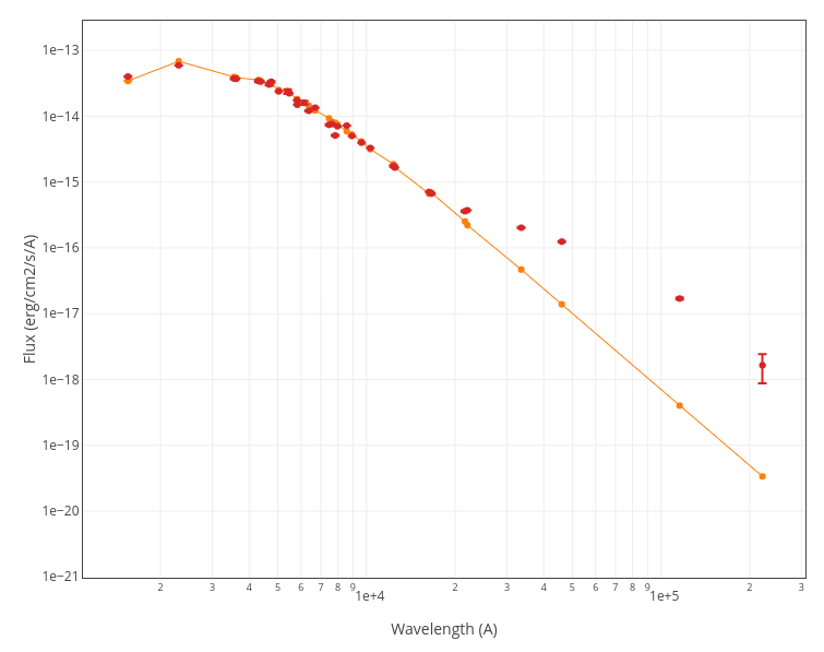
A typical case could be a SED with a clear infrared excess where we could have two clear contributions: the flux from a somewhat hotter object for the main part of the SED (in orange in the plot), and the flux coming from a colder object (cold star, dust...) for the infrared excess (in blue in the plot).
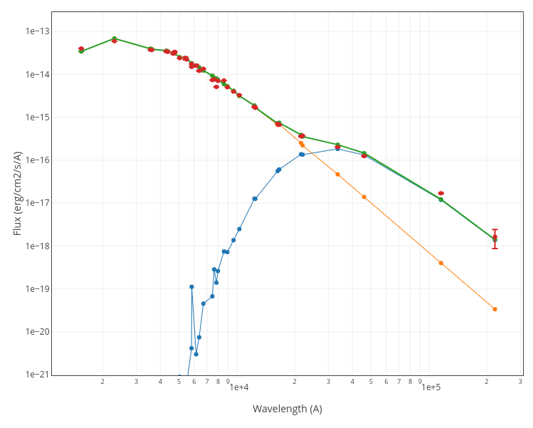
Binary Fit procedure
We can write this down as the fact that we want to represent the observed flux as the linear combination of two different models (the fluxes coming from two different objects), that is: $$ {\rm F}_{\rm obs}(x) \sim A \ {\rm F}_{\rm a}(x) + B \ {\rm F}_{\rm b}(x) $$
We know the observed fluxes ${\rm F}_{\rm obs}(x)$, and we know what theoretical grids to use for objects a and b (these are inputs from the user). We need to find the best parameters for each theoretical model and both dilution factors $A$ and $B$.
The method to do this, and estimate model parameters and A and B, is trying to minimize $\chi^2$ defined as: $$\chi^2 = \sum_x \left(\frac{A \ {\rm F}_{\rm a}(x) + B \ {\rm F}_{\rm b}(x) - {\rm F}_{\rm obs}(x)}{\Delta{\rm F}_{\rm obs}(x)}\right)^2 $$
Most of the explanations given in the chi-square model fit section are also valid for the binary fit. But there are very important differences.
We will focus here mostly in those aspects that are specific of the binary fit.
In the case of the one model chi-square typical fit, VOSA compares the observed SED with the synthetic photometry of all the models in the grid, calculates the best $M_d$ for each case and chooses the model so that chi-square is minimal. And this process, trying all the posible model parameter space, is quite deterministic as $M_d$ is calculated for each case, not estimated, fitted, etc, but calculated as one of the fit results.
But this is imposible for the binary fit. Here we can calculate one of the two dilution factors ($A$ or $B$) but we need to estimate the other one in a different way. And there is no deterministic way in which we can calculate all the parameters. For instance, if we rewrite our equation above as: $$ {\rm F}_{\rm obs}(x) \sim A \ \left( \ {\rm F}_{\rm a}(x) + R_{\rm f} \ {\rm F}_{\rm b}(x) \ \right) $$
we can make a loop through all the models (a and b) parameter space, try/estimate a value of $R_{\rm f}$, and then calculate the corresponding value for $A$. And we will have the best fit for that "estimation".
but we will never be sure that we have chosen the best posible value for $R_{\rm f}$.
In most of the cases, the success of the binary fit process relies in a good estimation of $R_{\rm f}$ (then, a loop of values around that estimation could help to refine the results).
We are going to explain briefly the algorithm used by VOSA to estimate the best binary fit parameters.
VOSA Binary Fit algorithm
There are several posible ways to implement this process. After many tests we have chosen the one explained here as a compromise of the time and resources used by the process and the accuracy of the results. You can get an analysis of the quality of the results obtained at the Binary Fit Quality section. And, please, remember not to use the binary fit as a black box that you can use and trust with your eyes closed.Remember that the main equation can be writen as: $$ {\rm F}_{\rm obs}(x) \sim A \ \left( \ {\rm F}_{\rm a}(x) + R_{\rm f} \ {\rm F}_{\rm b}(x) \ \right) $$
1.- Loop in models parameters space.
we try all the posible parameter values for both models (a and b). For instance, just to simplify the notation, we can imagine that the only parameter for these grids is the temperature and, thus, we try all the posible pairs (Teff$_{\rm a}$, Teff$_{\rm b}$).For each of these pairs we need to estimate a value of $R_{\rm f}$ (and $A$) that we think that will make sense.
To do this first estimation we need two equations to obtain values for A and B (or, actually, A and $R_{\rm f}$).
To get these two equations we take two different sets of points in the observed SED. For instance, one of them starting at short wavelengths and the other, on the contrary, starting at the longest wavelengths.
There are different approaches that we could use here, depending of the size of the sets and other conditions. But we have chosen one of the simplest ones:
- Use the equation above (the full linear combinaton of both models) and require that it fits well both the first and last points of the observed SED. That is, we use a set size = 1 for both SED ends.
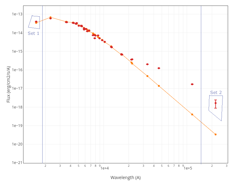
We can thus apply the corresponding equations and, for each point in the model parameter space, we get a first estimation of ($A$ and $R_{\rm f}$) as the values that fit well sets 1 and 2.
(teff$_{\rm a}$, teff$_{\rm b}$...)$_i$ $\Rightarrow$ (A,$R_{\rm f,estim}$)$_i$
(teff$_{\rm a}$, teff$_{\rm b}$...)$_j$ $\Rightarrow$ (A,$R_{\rm f,estim}$)$_j$
...
1.- Loop around first estimation.
After the first estimations, for each point in the model parameter space (teff$_{\rm a}$, teff$_{\rm b}$...)$_i$ , we define an interval of possible values of $R_{\rm f}$ ($R_{\rm f,min}$...$R_{\rm f,estim}$...$R_{\rm f,max}$) around this first estimate and we check if the global value of $\chi^2$ (using the full combination of models over the complete observed SED) improves when making a loop around the first estimation. In this way, for each pair of models we obtain a series of: (teff$_{\rm a}$, teff$_{\rm b}$...)$_i$ $\Rightarrow$ (A,$R_{\rm f,best}$)$_i$ $\Rightarrow$ $\chi^2_i$
(teff$_{\rm a}$, teff$_{\rm b}$...)$_j$ $\Rightarrow$ (A,$R_{\rm f,best}$)$_j$ $\Rightarrow$ $\chi^2_j$
...
And we finally select the one that gives the smallest value of $\chi^2$. And the corresponding values for model parameters, A and $R_{\rm f}$ that lead to this best fit.
(teff$_{\rm a}$, teff$_{\rm b}$...)$_{Best}$ $\Rightarrow$ (A,$R_{\rm f,Best}$)$_i$ $\Rightarrow$ $\chi^2_{Best}$
These are the values that will be returned by the binary fit process.
HR diagram
VOSA offers the option to estimate values for the age and the mass of the objects. In order to do that, the (Teff,log(L)) values obtained from the chi-square fit are used as starting points for interpolating collections of theoretical isochrones and evolutionary tracks obtained from the VO. Then, a HR diagram is displayed showing the data points, isochrones and evolutionary tracks.
For each object, only the theoretical isochrones and evolutionary tracks more adequate to the model that best fits the observed photometry are used in the process. For instance, in the case where this model is "Kurucz" the Siess isochrones are used.
In the case that several collections are used (because we use one for some objects and another one for other objects) a HR plot will be generated for each collection, showing the isochrones, tracks and the points corresponding to the objects analysed using that collection.
You can play with the plots, decide to plot more or less information, locate the objects in it, etc.
Error estimation
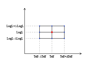
In order to make an error estimation, the errors coming from the chi-square fit for Teff and LogL are used to generate a small grid with 9 points.
For each of these 9 points we make the interpolation as explained below.
The final values for (Age,Mass) will be the ones obtained for the point (Teff,LogL). But in some cases, the interpolated value of Age or Mass is different for some of the other 8 points. Thus, in the results table we show the minimum and maximum value obtained for each parameter when using any of the 9 points in this small grid.
Interpolation
(Below, all the explanations are given for the case of obtaining an estimation of the object age interpolating on isochrones. Everything is valid also for the case of obtaining an estimation of the mass interpolating on evolutionary tracks.)
The interpolation between isochrones involves to find the two closer isochrones to the (Teff,log(L)) point (one to each side of the point), calculate the distance from the point to each of the curves and, then evaluate a weighted average between the values of t for each isochrone.
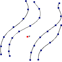 |
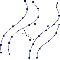 |
$t=\frac{t_2 D_1+t_1 D_2}{D_1+D_2}$ |
In order to do this it is necessary to design an algorithm able to estimate the distance from a point to a curve defined by discrete points (note that we do not have an analytical curve but just a series of points that are assumed to define a curve).
Distance from a point to a curve
1.-The main method that we use to estimate the distance form the point to an isochrone is as follows:
- First, given the point P (Teff,log(L)) find the closest point in the curve (point P1 at a distance D1)
- Second, find the projection of P to the line defined by P1 and either the next point in the curve or the prior one.
- If either of the projections lies into the interval defined by the two points (P1 and P2), then calculate the distance from the point P to the projection.
- This value will be taken as the distance from P to the isochrone.
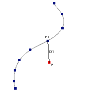 |
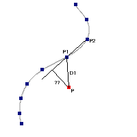 |
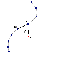 |
2.-In some cases, it is not possible to use the above method because none of the proyections lie inside the interval between the two points that define the line.
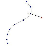 |
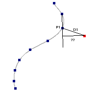 |
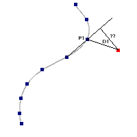 |
When that is the case, we can estimate the distance to the curve as the distance D1 from P to the closest point in the curve P1
Note that we consider this a worse approximation in general. Actually it is highly probable to be bad when P1 is the fist or last point in the curve.
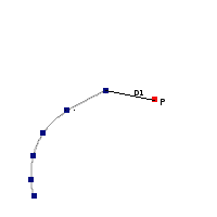 |
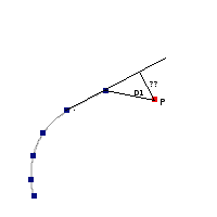 |
That is why we this method will only be used if the first one fails and if the closest point P1 is not the fist or last point in the curve.
Interpolated value for the age
If we have been able to find a curve on each side of the point P and the distance from that point to each curve, we can In some cases, we are able to determine only the distance to one curve, but we know that there exist an isochrone on each side of the point. If that happens we just show a range of values for the age using the ones corresponding to each isochrone as lower and upper limits.
Finally, if the point lies outside the area covered by the isochrones, we do not even try to estimate a value for the age or the mass of the object.
Whenever we are not able to find a value for the age or the mass of an object or it has been determined using a worse approximation that the one that we consider the best (See above) a flag is shown right to the value. These are the possible flags and their meanings:
We have made a chi-square model fit for a set of objects. The best fit model for all the objects was BT-Settl-CIFIST. Thus, when we enter the "HR diagram" tab we see the collection of isochrones and tracks that is going to be used as default for all the objects: BHAC15.
But we can click in the "click to add more options" link to change the default behaviour.
When we click the link a new form opens that allows to choose different isochrones/tracks collections depending on the Teff and Lbol values of each object. For instance, in this case we configure:
Take into account that if some object meets several conditions (for instance, Teff<=3800K and Lbol >= 0.75) priority will be assigned from bottom to top, being the default the last choice (that is, in this case, Parsec 1.2 will be used).
When we click the "Continue" button, we will see the available ranges of values (age and mass) available for each of the choosen collections. We could play with the ranges of parameters, restricting the values of the age and mass to be considered in the analysis. But we prefer to keep the full range and click the "Make the HR Diagram" button.
The interpolation process, to obtain the best values (and ranges) for the age and mass of each object, is performed asynchronously so that you don't need to stay in front of the computer waiting for the results. You can close your browser and come back later. If the process is not finished, VOSA will give you some estimation of the status of the operation and the remaining time.
When the process is finished, you can see the list of objects with the interpolation results, and three HR plots, one for each collection of isochrones and tracks.
If you click in any graph, VOSA will locate the object closest to the click point and will show you its properties.
If, instead, you click on one object name in the list, VOSA will locate that object in the corresponding graph.
You also can play with the plots. There are options to zoom to the objects range or to the models range. Other options allow you to define the exact range of each coordinate. And you also can decide what isochrones or tracks you want to display.
In some cases, there are points in the SED marked as "upper limit" (because VO catalogs label them as that, or because the user has marked the corresponding option at the 'edit SED' tab.
These points are displayed in the SED plots with a triangle instead of a dot.
Photometric points marked as "upper limit" are taken into account for the chi2 and bayes analysis but in a different way than the other points.
To perform the corresponding fit an upper limit with flux ${\rm F}_{uplim}$ is included in the SED to fit as:
$${\rm Flx} = 0 $$
$$\Delta{\rm Flx} = {\rm F}_{uplim}$$
When the chi2 model fit is performed with the option of estimating parameter uncertainties using a statistical approach, a 100 iteration Monte Carlo simulation is done. In this case, 100 different virtual SEDs are generated introducing a gaussian random noise for each photometric point (proportional to the observational error). But for the upper limits, in the virtual SEDs a random flux will be generated between 0 and ${\rm F}_{uplim}$ following a uniform random distribution.
In the case that the user does not want to treat upperlimits in this way, there is the option to perform the chi2 fit ignoring upperlimits. In that case, these points will not be taken into account at all during the process.
When you visualize the individual fit results, you will see what points are upperlimits and if they have been used for the fit or not.
We have obtained a set of N different values for the quantity X: $\{X_i\}$.
The values can be grouped in different bins, so that we have a set of ordered pairs {value,frequency}.
$$ \{X_i,Freq(X_i)\}$$
$${\rm with } \ X_i > X_{i-1}$$
A percentile is the value below which a given percentage of observations in a group of observations fall.
Let's define some notations for the case of grouped values:
$N = \sum Freq(X_i)$ (total number of values)
$ S_n = \sum_{i<=n} Freq(X_i) $ (cumulated sum of frequencies up to the n-th bin)
$ S_k = k * N/100$ is the cumulated sum of values corresponding to the k-th percentile (for instance, if we are looking for $P_{73}$ in a distribution with 1000 values, $S_k=730$)
When we are looking for the k-th percentile, and $S_n = S_k$, then $P_k = X_n$.
But if often happens that $S_{i-1} < S_k$ and $S_i > S_k$. In this case, the k-th percentile can be calculated using a linear interpolation:
$$P_k = X_{n-1} + (X_n - X_{n-1}) \frac{S_k - S_{n-1}}{S_n - S_{n-1}} $$
The quartiles of a distribution are defined as the 25, 50 and 75 percentiles. That is:
$$Q_1 = P_{25}$$
$$Q_2 = P_{50}$$
$$Q_3 = P_{75}$$
The median is defined as the X value so that half the values in the distribution are smaller and the other half are larger. It can be said that it is the "medium point of the distribution".
In practice, it is defined as $P_{50}$.
$${\rm Median} = P_{50}$$
The mode is the value that appears most often in a set of data.
There are several tests that can be used to estimate if a given set of values corresponds to an underlying Normal distribution.
In VOSA we have implemented the Pearson's chi-squared goodness of fit test. Both at the Bayes analysis and the Chi2 model fit (when parameter uncertainties are estimated using a Monte Carlo method).
Pearson's chi-squared test
Pearson's chi-squared test uses a measure of goodness of fit which is the sum of differences between observed and expected outcome frequencies (that is, counts of observations), each squared and divided by the expectation:
$$ \chi ^{2} = \sum _{i=1}^{n} \frac{ (O_{i}-E_{i})^{2} }{E_{i}} $$
where:
The expected frequency is calculated by:
$$ E_{i} = N \cdot [ F(Y_{u}) - F(Y_{l}) ] $$
where:
Once obtained the value of $\chi^2$ we compare it to the chi-square distribution for the corresponding degrees of freedom and obtain a range of values for the probability that our values, $ \{X_i,Freq(X_i)\}$, can correspond to an underlying normal distribution.
See, for instance, Goodness of fit (at the Wikipedia) for more details.
VOSA generates many results that you can visualize, download in different formats or send to other VO applications using SAMP.
You can also get a log file with a summary of all the activities done in VOSA for each input file, and the references to all the services that have been relevant to obtain your results.
See more details about each of these points.
VOSA offers you the posibility of downloading all the results in several formats.
In order to get the available files, enter the 'Save results' panel.
You will see a form where you can select what results you want to download and in what formats. Obviously, if you haven't generated results of some type yet, they will not be available.
For instance, you can mark all the available options and click the "Retrieve" button.
VOSA will make a compressed tar file with all the information so that you can dowload it.
When you explore the tar file, you can see several folders containing files of different types. For instance:
There are files in different formats:
SAMP is a VO protocol that allows to share data between VO applications. It was initially designed to work between desktop applications but, thanks to Mark Taylor's sampjs library VOSA, being a web application, can share results with desktop applications too.
Thus, apart from just visualizing and downloading the final results, most of the tables can be broadcasted to any other VO application that is open in the final user computer and connected to the SAMP Hub. In particular, this is specially useful to send some results tables to Topcat for further analysis.
As far as you have an active SAMP Hub in your computer (for instance, if you have Topcat open) you will see a "Sent table to SAMP Hub" button in some of the VOSA results. For example, in a model fit, you can see it:
The SAMP Hub will request authorization to broadcast the file sent by VOSA: You can accept it safely.
The VO table sent by VOSA will be loaded into TopCat,
and you will be able to use Topcat functionalities to work with it.
VOSA uses external services, theoretical models and science inputs from different sources that you might want to cite or acknowledge if your research benefits from the work done by VOSA.
You can check the Credits section section to see a full list of all the credits.
But, depending on the work that you have done with your user file, you will probably have used only some of those services.
Whenever you download results files in the 'Save results' tab, you get two important files:
At any moment, you can check the 'Refs' tab to see a web version of the references file.
A summary of all the activities that you do in VOSA is saved in a log file that you can download together with the obtained results.
And, at any time, you can see a web version of this file in the 'Log' tab, with all the activities in reverse order (the last activity is shown first).
VOSA generates graphs for object SEDs, model fits, bayes analysis, HR diagram...
These graphs are generated and displayed in VOSA as simple PNG files.
But some versions of these graphs are also generated in postscript format and as .agr files.
For each plot, for instance, the SED of the HD99827 object, these files are generated:
Grace is a free WYSIWYG 2D plotting tool, developed initially for Unix-like operating systems but also ported to OS/2, Windows, etc.
It allows to play with graphics, customize lines, colors, axes, etc., and even apply some analysis options to the data sets.
VOSA generates a .agr version of every plot so that you can use Grace to customize the plot if you feel the need to do it, for instance, to include it in a publication.
You only need to open some of the .agr files generated by VOSA and you will see a plot very similar to the PNG version.
You have many options to customize the graph appearance. As a simple example, you can change the red circles to green triangles:
Once you are finished editing the graph, you can use the "File:Print Setup" dialog to specify how you want to save the plot, including PNG, EPS and other formats. Then, use the "File:Print" dialog to generate the final file.
Take a look to the Grace online help for details about how to use the many available options.
VOSA is a web application.
This means that you only need a web browser (Firefox, Chrome, Explorer...) and an internet connection to use it. You don't need to install anything else.
All the VOSA operations are performed in the VOSA servers, no computing is done in your own machine. So you will only need the amount of memory that the browser needs to display the results (usually small) and the disk space to finally download the results files if you want to do it.
In exchange, as all operations are done in the VOSA server, big processes can be an important load to the server specially when several users are submitting jobs at the same time. And, in web applications, you usually have to wait, with the browser open, to the process to finish so that the results are loaded in the web page. If the process is long, this can be a problem.
Whats more, the advent of new and more sensitive surveys providing photometry at many wavelength ranges and covering large sky areas (GAIA, GALEX, SDSS, 2MASS, UKIDSS, AKARI, WISE, VISTA...) is pushing astronomy towards a change of paradigm where small groups, and not only large consortia, need to analyze large multi-wavelength data sets as part of their everyday work.
Thus, to be ready to work with large samples of objects, we have redesigned VOSA architecture since version 5.0 so that, keeping the advantages of being a web application, the drawbacks are reduced.
Now VOSA works with a
distributed,
parallelized and
asynchronous architecture,with an
improved design for large files. See more details below.
Now, most of the VOSA calculations are not done in the VOSA server. VOSA submits them to a different server and waits for the results. This reduces very much the VOSA server load, that does not depend much on the number of jobs or the size of user files.
In the future this infrastructure could be upgraded so that VOSA can distribute jobs among different servers to balance the load.
VOSA is designed to work with files with lists of objects and make mostly the same operations to all of them.
But most VOSA calculations are now parallelized, so that it's not necessary to finish the work with one object to start the next one. The computation server organizes the jobs so that several of them are done in a parallel way, and collects the results once all the jobs are finished.
VOSA communicates with the computation server in an asynchronous way. That is, VOSA submits a process and does not wait for it to finish. From time to time, or because a user requests it, VOSA checks the status of the process and, when it is finished, downloads the results, makes the final necessary processing and presents them to the user.
The main advantage of this is that you, the final user, do not need to wait, with the browser open, to the end of the process. You don't depend on the stability of your internet connection either. You can start a process, close the computer and come back later to see how it is going. If it is finished you will see the results. If not, you will see the status of the process and an estimation of the remaining time.
Processes can be canceled at any time from the VOSA web interface.
The asynchronous behavior is visualized in a similar way in all VOSA processes.
When you submit a process (for instance, a model fit), VOSA gathers the information, submits it to the computing server and waits for a while to check if the process is going to end shortly. So, during a short while (some seconds) you see something like this:
If VOSA sees that the process is not going to finish almost immediately, it tells you that the process has been submited asynchronously and gives you information of its status and (when possible) some estimation of the remaining time
At this point you can close the computer if you want and come later again to the page to see how the operation goes.
You can cancel the process whenever you want. You just need to click the "Cancel" button. VOSA will ask you for confirmation. If you confirm it, the process will be canceled and you can restart it again, maybe with different options. If you don't confirm, the process will continue as it was.
Once the process is finished, VOSA downloads the needed information from the computing server and starts processing it (what could include, for instance, making some plots).
And, finally, the results are displayed.
A great deal of the VOSA capabilities depend on what we call the SVO Theory Data Server.
Another great part of the VOSA capabilities depend on external services, provided by different data centers and that are accessed by VOSA using Virtual Observatory (VO) protocols (ConeSearch, TAP and SSAP).
In particular, VOSA uses these services to search for objects properties (distance, extinction) and photometry.
SAMP is a VO protocol that allows to share data between VO applications. It was initially designed to work between desktop applications but, thanks to Mark Taylor's sampjs library VOSA, being a web application, can share results with desktop applications too.
Thus, apart from just visualizing and downloading the final results, most of the tables can be broadcasted to any other VO application that is open in the final user computer and connected to the SAMP Hub. In particular, this is specially useful to send some results tables to Topcat for further analysis.
See the SAMP section for more details.
For big user files containing thousands of objects, the plain visualization in a web page is not very useful. And, in some cases, it could even require a lot of memory and freeze or kill the web browser.
In order to avoid this problem, we have redesigned the presentation of large results tables implementing a customizable pagination form.
For instance, in the model fit, when there are many objects in the file you will see something like this:
In general, when there are many objects, you will not see the full list at once but only, for instance, the first 10 ones. And, together with that list, you will see a form where you can:
In some calculations performed by VOSA it is necesary to use values for certain physical constants. There are the values that we are using:
References: Why parallax errors in TGAS are larger in VOSA than those given by the catalogue?
How is the counterpart selected in the photometric catalogs?
If a photometric point has ΔFlux=0, how is this treated in the fit?
From magnitudes to fluxes: How does VOSA compute the error in flux from the error in the catalogue magnitudes?
Stromgren: Does Paunzen (2015; J/A+A/580/A23) supersede Hauck et al. (1997; II/215)?
Stromgren: Why, sometimes, the errors in flux associated to the photometric values of the Paunzen catalogue are larger than the rest of photometric points?
Stromgren: How do we go from the information available in Stromgren photometry catalogues (V, (b-y), m1, c1 and the respective errors) to the uvby magnitudes and the respective errors?
Which catalogues are included in the "info/refs.dat",
"info/refs.bibtex.bib" files, automatically generated when the results
are downloaded?
On the contrary, if the target has no counterpart in a catalogue, this
catalogue will not be included in those files.
Why does Gaia photometry appear to be clearly outside the SED even for good fits? This is just an example of the fact that you shouldn't try to fit observed photometry using the theoretical spectrum directly. You need to compare the observed photometry with the synthetic one calculated using the theoretical spectra and the filter passband.
Why does it happen that, in particular cases, SDSS fluxes are negative? Magnitudes should not produce negative fluxes but SDSS magnitudes are not the typical pogson ones but asinh "laptitudes" and the conversion formula that we apply is:
$${\rm Flx} = {\rm F}_0 \ 10^{-{\rm mag}/2.5} [ 1-{\rm b}^2 * 10^{2 {\rm mag}/2.5}]$$
this shouldn't produce negative fluxes either but it can happen and, when it happens, VOSA rejects the corresponding flux values as bad.
You can take a look to the filter information for more details and the particular parameter values for each SDSS filter.
The Av/Teff degeneracy: What is the combined effect of extinction and effective temperature in the SED?
This effect is considerably reduced when the distance to the object is known so that you can restrict to small values of Av.
This can be clearly seen if the Bayes analysis is performed (see figures). In this case, the best effective temperature calculated using the chi2 fit may not be the good one from the physical point of view.
Why The fit process takes much longer when you decide to include the model spectrum in the fit plots?
Thus, if you have a VOSA file with thousands of objects, don't check the "Include model spectrum in fit plots?" unless you really need that.
Why the theoretical models that best fit for each object (that is, already multiplied by Md and scaled to the observational points) are not included in the list of VOSA products, for instance as a lambda, flux table?
The theoretical spectra are not included in the list fo VOSA products mainly because of their size. For instance, the size of a single BT-Settl spectrum is 8 MB.
The best way to download the theoretical spectrum that best fits the data is going to the "Best fit" table of results. The last column of the table, titled "Data VOTables" gives you a link to get the full theoretical spectrum corresponding to each object fit.
WARNING: As these files may be large, and in order to avoid web browser crashes, it is advisable to save them using the "Save as" option (right buttom of the mouse) instead of directly cliking on the link.
Besides this, as a side trick, take into account that .agr files for the plots with the fit results contain a resampled version (lower resolution) of the theoretical spectrum if you have chosen to include spectra in the plots. These are ascii files, and you can find the spectrum at the end of the file as the table with the largest number of points.
In this section we provide a detailed example on how to use this application. We will consider a case where the user has 2MASS, CFHT and IRAC photometry for ten objects and will show the complete VOSA workflow, step by step. This example is just a subset of the physical case studied in Bayo, A., Rodrigo, C., Barrado y Navascués, D., Solano, E., Gutiérrez, R., Morales-Calderón, M., Allard, F. 2008, A&A 492..277B
We consider two objects labelled as LOri001 and LOri002. For each of them we need: We also have some observed photometry for these objects, corresponding to:
The observed magnitudes (and errors where available) are like:
With this information we can build a file in the data format required by VOSA. Note that we have writen a line for each photometric value that we have. In each line: Take into account that, for a general case, only the first column (the object label) is mandatory. All the other ones can be writen as '---'. Once we have an ascii file like this, we can go to the next step: uploading the file. Once the data file is ready, go to the Upload File tab and click in the Browse button (take into account that, depending on your browser language, the displayed word could be different). A new window will open so that you can browse your file system and select the data file to upload. Then, you must fill in the form. Give a description to the file and make sure that you mark the Magnitudes option because the user photometry, in this case, is given in magnitudes. Then click in the Upload button. If everything goes ok, a ... has been successfully uploaded message will appear. You then click in the "Continue" link and see the main info about the uploaded file and some options.
Now, you can already start working with this file. But it is a very good idea to check if VOSA has understood all the info that you have uploaded. Just click the "Show Objects" button and, if everything has gone ok, you will see the information about the particular objects.
If something has gone wrong, delete the file, check its contents and try to upload it again. We have the option of consulting some VO catalogues to look for more photometry for the objects in our sample. In order to do that, we enter the "VO Phot" tab. You can choose among several catalogues. Only the closest result will be shown in the results table. Thus, it does not make sense to use a large search radius; it only will result in a longer response time. In this case, we fix all the search radius to 5 arcsecs for each catalogue and click in the "Query selected services" button. When the search is finished we see that some data have been found in three catalogs: SDSS, 2MASS and WISE, and these data are incorporated to our objects SEDs. Some of them (several of the ones corresponding to WISE.W4) are only upper limits, and they will not be used in the fits.
Now we could go to the "SED" tab to inspect (and, eventually, edit) the final SEDs for our objects.
You can see the information for each photometric data point. For instance, you see here that, for each of the 2MASS points, VOSA has averaged the user value (provided by us in the input file) and the one obtained from the 2MASS catalogue (in this case, this does not produce any effect because both values are identical).
We could make changes here, exclude some points, etc. But we are happy with the final SEDs so we will go to the next workflow step.
The determination of physical parameters of astronomical objects from observational data is
frequently linked with the use of theoretical models as templates. The use, in the traditional way, of this methodology can easily become tedious and even
unfeasible when applied to a large amount of data. VOSA uses VO methodologies to authomatically fit
several collections of theoretical models to the observed photometry for different objects When we access the Chi-2: Model Fit tab we see a form with the available theoretical models, so that we can choose what ones we want to use in the fit. In this case we decide to try Kurucz and BT-Settl-CIFIST models. Thus, we mark them and click in the "Next: Select model params" button. For each of the models, we see a form with the parameters for each model and the available range of values for each of them. We choose the ranges that best fit our case and then click the "Next: Make the fit" button. The fit process is performed asynchronously so that you don't need to stay in front of the computer waiting for the search results. You can close your browser and come back later. If the fit is not finished, VOSA will give you some estimation of the status of the operation and the remaining time.
When the process finishes VOSA shows us a list with the best fit model (that is, the one with a smaller value for the reduced chi-2) for each object. Optionally you can also see the best fit plots, with the observed SED and the corresponding synthetic photometry for the best fit model. If you click one object name, you can see the 5 best fits for each collection of models. And clicking on the "See" link on the right of each fit, you can see the details about it.
Sometimes the fit with the best Χ2 is not the one that the user considers the best one, maybe for physical reasons, taking into account the obtained values of the parameters, or maybe because one prefers a model that fits better some of the points even having a larger Χ2... Whatever the reason, we have the option to mark as Best the model that we prefer. In order to do that we just click in the Best link at the right of the model that we prefer. In this case we choose the third one for LOri001. And when we go back to the bestfit list, we see that the fit that we have just selected is listed as the best one for LOri001.
At any time, you can move your mouse over each of the table headers and a window will appear with short explanation of the concept represented in that column. In this process we have been able to estimate some physical parameters for our objects. The models have given us the effective temperature, surface gravity and metallicity. Also, the total flux of the objects can be estimated using the model for those areas of the spectrum not covered by the observed photometry. And finally, using the distance given by user, the application estimates the bolometric luminosity of the object. The model chi-2 fit gives us the parameters for the best fit model. But a Bayesian analysis uses all the fits to estimate the probability fo each parameter value.
In order to try this option, we enter the "Model Bayes Analysis" tab and we see a form with the available theoretical models, so that we can choose what ones we want to use in the fit. In this case we decide to try Kurucz and BT-Settl-CIFIST models as we did in the chi-2 fit. Thus, we mark them and click in the "Next: Select model params" button. For each of the models, we see a form with the parameters for each model and the available range of values for each of them. We choose the ranges that best fit our case and then click the "Next: Make the fit" button. The fit and analysis process is performed asynchronously so that you don't need to stay in front of the computer waiting for the search results. You can close your browser and come back later. If the fit is not finished, VOSA will give you some estimation of the status of the operation and the remaining time.
When the process finishes VOSA shows us a list with, for each object and each model collection, the most probable value for each parameter and its probability.
And, if we click in one object name, we see a detailed information for that object with the probability of each parameter value and the corresponding plots.
In order to estimate values for the mass and age of our objects, we use collections of isochrones and evolutionary tracks to build a HR diagram. First, we access the HR diagram tab.
In order to build an HR diagram VOSA uses the available collection of isochrones and evolutionary tracks more adequate for the best model fit for each object.
In this case, the best fit model is Kurucz for some objects and BT-Settl-CIFIST for some others. For the objects with a Kurucz best fit, we will use the Siess isochrones and tracks. For those with a BT-Settl-CIFIST we will use the BHAC15 ones.
When we click the "See list of objects" link, we can see the list of objects that will correspond to each collection of models.
When we click in the Make HR diagram button VOSA builds and HR diagram (one for each model collection) and, interpolating among the isochrones and evolutionary tracks, estimates values for both the age and the mass of our objects. If you click in one of the object names VOSA will locate it in the corresponding plot. If you click in some point of one of the plots, VOSA will identify the closer object. You can play with the plots in a number of ways.
Interpolating the isochrones and tracks VOSA has estimated values for the age and mass of most of our objects. We have now more physical properties for them:
Finally we want to download all the results that we have obtained in this session.
We access the Save Results tab and we see a form with all the information that is available to download. Obviously, we cannot download anything related to Template fit or Template bayes analysis because we haven't tried those options in this case.
We mark all the available options and click the "Retrieve" button.
VOSA will make a compressed tar file with all the information so that we can dowload it.
When you explore the tar file, you can see several folders containing files of different types. For instance:
Date of this test: 2021/06/23
To assess the performance of VOSA to estimate effective temperatures of FGK stars, we have made use of the Elodie library (v3.1) (1389 objects).
First, we kept only entries in Elodie having a quality flag=4 ("excellent") in effective temperatures (159 objects)
Then, we cross-matched with the Gaia EDR3 catalogue looking for counterparts in 5arcsec. In order to avoid extinction - effective temperature degeneracies, we kept objects with parallaxes > 10 mas and relative errors < 20% (parallax_error/parallax < 0.2). After this, we kept 127 objects.
The observational SED of these objects were built gathering photometry from the following catalogues: SLOAN DR12, APASS9, Gaia EDR3, Pan-Starrs DR2, and 2MASS. Also the following grid of models were used: Kurucz ODFNEW/NOVER, alpha:0.0; Kurucz ODFNEW/NOVER, alpha0.4; BT-Settl, BT-Settl (CIFITS). Only objects with good SED fitting (vgfb < 12) were considered for the comparion.
Kurucz model, alpha: 0.0.
Teff_VOSA - Teff_Elodie: 6.43 ± 102.77 K (42 objects)
Kurucz model, alpha: 0.4.
Teff_VOSA - Teff_Elodie: 18.33 ± 96.57 K (42 objects)
BT-Settl.
Teff_VOSA - Teff_Elodie: 50.47 ± 113.42 K (42 objects)
BT-Settl-CIFIST.
Teff_VOSA - Teff_Elodie: 15.68 ± 99.32 K (42 objects)
We can see how, for the four collections of models, VOSA estimates effective temperatures close to those given in Elodie. Only to mention that temperatures estimated using BT-Settl are slightly lower, in particular at Teff < 5200K.
The position in the H-R diagram of the 42 objects used in the comparison is given below.
The forty-two objects used in the comparison are the following:
To assess the performance of VOSA at high temperatures we have used the compilation of sdO stars made by Stroeer et al. (2007 A&A, 462, 269)
For our analysis we have selected only those sdO targets not flagged as "outliers" in effective temperature (Table1 of the paper). Then, for these targets, the observational SED has been built using photometry (GALEX, CMC-14, 2MASS) retrieved from VO services using VOSA. The following criteria were adopted:
An average value of Teff (VOSA)-Teff (Stroeer)=2800 ± 6700K is found for a sample of 14 objects.
Date of this test: 2017/05/16
We compare the results in Yee et al. with the fit results obtained by VOSA.
Only objects with good fit (vgfb<=12) and sigma<200K in the Bayesian fitting are considered (155 objects).
Using Kurucz model we find:
Teff (Yee) - Teff(VOSA)
Only objects with good fit (vgfb<=12) and sigma<0.3dex in the Bayesian fitting are considered (38 objects).
Using Kurucz model we find:
logg (Yee) - logg (VOSA)
But if we use BT-Settl instead of Kurucz, the situation is the reverse, with the gravity values computed by VOSA systematically higher than those given in the paper (28 objects have been used this time).
Only objects with good fit (vgfb<=12) and sigma<0.3dex in the Bayesian fitting are considered (141 objects).
Using Kurucz model we find:
[M/H] (Yee) - [M/H] (VOSA)
A similar result is obtained is BT-Settl is used:
Only objects with good fit (vgfb<=12) and errors in Parallaxes (TGAS) < 10% (190 objects).
Excellent agreement between the distances used in the paper and those used in VOSA (from TGAS).
Radius1 (VOSA); defined by: Md = (R/D)^2
Using Kurucz model we find:
Radius1 (Yee) - Radius1 (VOSA)
Radius2 (VOSA); defined by: Lbol = 4 * pi * R^2 * σ * Teff^4
Using Kurucz model we find:
Radius2 (Yee) - Radius2 (VOSA)
Similar plots are obtained if BT-Settl models are used instead.
Only objects with good fit (vgfb<=12). 54 objects (restricted to masses below 1.4 Msun)
BTSettl isochrones and tracks.
Excellent agreement for subsolar masses. Masses over 1Msun are overestimated in VOSA-BTSettl.
Mass(Yee) - Mass (VOSA_BTSettl)
Similar results are obtained if the BTSettl-CFITS isochrones and tracks are used:
Date of this test: 2017/07/18 (by Miriam Cortés Contreras)
We compare the results in Lindgren & Heiter 2017 (here-after LH17) with the fit results obtained with VOSA.
Efective temperatures computed by VOSA are in agreement with those
given in LH17. On average, LH17 temperatures are systematically
higher by less than 100K both for BT-Settl and CIFITS. Standard
deviations are below 150 K in both cases.
Below 3400 K, LH17 effective temperatures are larger (250 K and 450 K)
than those provided by BT-Settl. This trend does not appear if CIFITS
models are used. Anyway, a larger number of objects would be neces-
sary to confirm this result.
As expected from the minor contribution of these parameters to the
SED shape, the values obtained from VOSA are affected by large uncertainties and, thus, are not reliable.
There are not significant differences between the radii derived using BT-Settl or BT-Settl CIFIST models and both are in very good agreement
with the values derived by LH17.
While masses directly derived from M = gR 2 /G are not reliable due
to the large uncertainties associated to the surface gravities estimated
with VOSA, those obtained using the BT-Settl and BHAC isochrones
are in reasonable agreement with the ones obtained in LH17. The
agreement is slightly worse if the BHAC isochrones are used.
For comparison and to assess whether the parameters obtained with VOSA
are model-dependent, we performed this analysis using two models: BT-Settl
and BT-Settl CIFIST. One of the sixteen stars has not enough photometric
data. Thus, this analysis was carried out for the fifteen remaining stars.
Effective Temperatures
Mean(Teff(LH17) - Teff(VOSA)) = 92.9 K; std = 132.4 K
Mean(Teff(LH17) - Teff(VOSA)) = 86.3 K; std = 117.2 K
Both models give consistent values for the effective temperature.
Metallicity
Mean(Metallicity(LH17) - Metallicity(VOSA)) = 0.18; std= 0.38
BT-Settl does not provide good results for the metallicities.
Surface gravity
Mean(log g(LH17) - log g(VOSA)) = 0.05; std= 0.61
Mean(log g(LH17) - log g(VOSA)) = -0.48; std = 0.35
Surface gravities provided by VOSA are not consistent with the values
given in the paper. Using BT-Settl we obtain higher values for stars with the
lowest gravities in LH17 and lower values for the stars with highest gravities
(see Fig. 4). On the other hand, this does not happen using BT-Settl CIFIST but we obtain significantly higher values.
Radii and masses
VOSA computes two stellar radii from two different equations:
$$ M_d = (R_1 /D)$$
$$ L_{\rm bol} = 4\pi R_2^2 \ \sigma \ T_{\rm eff}^4$$
where M d is the proportionality factor used to fit the model to the observations, D is the distance and $\sigma$ is the Stephan-Boltzmann constant.
From $R_1$ and $R_2$ , VOSA provides also stellar masses by applying:
$$ g = \frac{GM}{R^2}$$
Since the surface gravities provided by VOSA do not agree with those
given in the paper, we do not expect consistent masses either. In any case,
we performed for the masses the same analysis as for the radii and will derive
proper masses from the HR diagram.
There are not significant differences between the radii derived using BT-
Settl or BT-Settl CIFIST models. Similar radii are obtained from Eqs. 1 and 2 and both are in very good agreement with the values derived by LH17.
On the contrary, masses are not consistent with the masses expected
for cool dwarfs and, hence, do not agree with those given in the paper, as
expected from the log g values obtained with VOSA.
Masses from HRD
Mean(Mass(LH17) - Mass(VOSA)) = 0.07; std = 0.06
Two K dwarfs lie outside the area covered by the isochrone. With
a few exceptions, we found good agreement between values for the
thirteen remaining dwarfs.
Mean(Mass(LH17) - Mass(VOSA)) = 0.08; std = 0.08
In this case, only one K dwarf lies outside the area covered by the
isochrone. The agreement with the masses in LH17 is worse using
BHAC isochrones.
Date of this test: 2017/09/22 (by Miriam Cortés Contreras)
We compare the effective temperatures and luminosities derived by Carlos Cifuentes San Román (Master thesis, Sept. 2017, Universidad Complutense de Madrid; hereafter CCSR), and the effective temperatures from Passeger et al. in prep. (hereafter Pass17) with the fit results obtained with VOSA.
VOSA provides effective temperatures using BT-Settl models in agreement with the estimated values of CCSR within 200 K. The comparison with the effective temperatures computed by Pass17 results in a higher dispersion. This differences are explained by the differences among CCSR's and Pass17's temperatures (the relation between them gives a correlation coefficient of r=0.88).
Excellent agreement between the bolometric luminosities provided by VOSA and CCSR's.
Of the 48 stars in this study, five have not enough photometric points retrieved by VOSA for the fit.
To give an idea of the temperatures used for the analysis, the difference between them has a mean value of 58 K and a standard deviation of 111 K.
Mean(Teff (CCSR) - Teff (VOSA)) = -7 K; std = 210 K
Effective temperatures provided by VOSA are in agreement with those derived by CCSR with one exception which effective temperature is 1000 K higher than estimated by CCSR. Fig. 1.
Mean(Teff (Pass17) - Teff (VOSA)) = -21 K; std = 334 K
In this case, the concordance between temperatures is slightly worse, but also consistent. On average, VOSA provides higher values. Fig. 2.
In CCSR, luminosities were derived from two different approaches: via Simpson's rule and Trapezoidal rule. The difference between them has a mean value of 0.00008 Lsun and, therefore, the comparison will be carried out using the luminosities obtained via Trapezoidal rule. The comparison with those obtained via Simpson's rule would be analogue.
Mean(L (CCSR) - L(VOSA)) = -0.002 Lsun, std= 0.004Lsun.
The estimated luminosities are in very good agreement. Fig. 3.
Date of this test: 2017/09/21 (by Miriam Cortés Contreras)
We compare the results in Rajpurohit et al. 2017, arXiv170806211R (hereafter Ra17) with the fit results obtained with VOSA.
Efective temperatures computed by VOSA are in agreement with those given by Rajpurohit et al. (2017) in the studied range from 3000 to 4000 K, with some dispersion towards higher values between 3100 and 3300 K. On average, temperatures provided by VOSA are systematically lower by less than 100 K and standard deviations are below 150 K for both BT-Settl and CIFIST models.
Metallicities and surface gravities provided by VOSA are not reliable due to the minor contribution of these parameters to the SED shape.
We performed this analysis using BT-Settl models and used the more recent BT-Settl CIFIST models for comparison.
Of the 45 M dwarfs of the analysis, only four had parallactic distances retrieved from VO services and another six had not enough photometric data for the fit.
Mean(Teff (Ra17) - Teff (VOSA)) = 20.5 K; std = 111.4 K
Mean(Teff (Ra17) - Teff (VOSA)) = 18.0 K; std = 110.6 K
Both models provide quite similar values for the effective temperatures and are overall consistent within the errorbars with those given in Rajpurojit et al. (2017).
Mean(Metallicity(Ra17) - Metallicity(VOSA)) = -0.19; std= 0.41
No good determination of the metallicities using VOSA. On average, metallicities obtained using BT-Settl models differ with the values given by Rajpurohit et al. (2017) by more than 7σ.
Mean(logg (Ra17) - logg (VOSA)) = 0.36; std= 0.65
Mean(logg (Ra17) - logg (VOSA)) = 0.29; std = 0.56
The surface gravities given by VOSA strongly differ with those given by Rajpurohit et al. (2017) for near half of the analyzed sample. Hence, these values are not trustworthy.
Date of this test: 2016/10/08
Sample: 100 good sources.
Conclusion: APASS fluxes are systematically higher in both bands (typically 10%) (Figures 3,4).
Date of this test: 2020/06/01
Sample: We have taken a sample of 664 objects in common in both catalogues and have compared the fluxes provided by VOSA.
Methodology:
Conclusions:
RA: 10.57339; DEC: 5.34662
Date of this test: 2017/05/08
Sample: we have taken a good quality sample of 784 objects in common in both catalogues and have compared the fluxes provided by VOSA.
Methodology:
Conclusions:
g band
r band
z band
Date of this test: 2016/10/08
We have taken a sample of "good" (no quality flags) sample of 200 objects in common in both catalogues and have compared the fluxes provided by VOSA.
Methodology
Conclusions:
Date of this test: 2017/05/08
Sample: we have taken a good quality sample of 200 objects in common in both catalogues and have compared the fluxes provided by VOSA.
Methodology:
Conclusions:
g band
r band
i band
z band (No comparison was performed due to the significant differences both in wavelength coverage and shape between the two filters).
Date of this test: 2017/05/08
Sample: we have taken a good quality sample of 119 objects in common in both catalogues and have compared the fluxes provided by VOSA.
Methodology:
Conclusions:
u band
g band
r band
i band
Date of this test: 2019/08/21 (by Miriam Cortés Contreras)
862 sources remain.
Observed vs. Model
We compared the observed fluxes in each of the five bands of XMM-SUSS4.1
with the theoretical fluxes predicted by the model in Figures 1 and 2.
XMM vs. GALEX and APASS
We compared the UVM2 band with the NUV filter of GALEX. Figure 3 shows
the normalized transmission curves of the filters, the comparison between
observed fluxes and the distribution of the flux ratio.
In the optical, we compared the B and V bands with the B and V filters
of APASS. Figures 4 and 5 show the normalized transmission curves of the
filters, the comparison between observed fluxes and the distribution of the
flux ratio.
Regarding the flux comparison with other filters, fluxes in the UVM2
band are systematically higher when comparing UVM2 with NUV. In the
optical, the comparison between the B and V bands of XMM and APASS
show very good agreement. (see Table 2).
An example of a SED fitted with BT-Settl using these bands is shown in
Figure 6. Date of this test: 2020/03/25
Goal: We want to check how the GALEX GR5/MIS (Bianchi et al. 2011) FUV and NUV fluxes fit in the overall SED.
Methodology
Conclusion:
Date of this test: 2020/03/25
Goal: We want to check how the GALEX GR6+7 (Bianchi et al. 2017) FUV and NUV fluxes fit in the overall SED.
Methodology
Conclusion:
The aim of this document is to present the results obtained from the tests carried out to assess the performance of the binary fit functionality implemented in VOSA and the accuracy of the derived physical parameters, in particular effective temperatures.
Firstly, we evaluated the effective temperatures estimated by VOSA for different types of single stars (FGKM spectral types and white dwarfs) using different collections of theoretical models (BT-Settl, BT-Settl CIFIST and Koester). Once the reliability of the results obtained for single stars was confirmed we, then, use those theoretical models to fit two-body SEDs. It is very important to be aware of the limitations and caveats found in this assessment of the two-body SED fitting functionality of VOSA and do not blindly use it.
Individual objects:
After the filtering we were left with 41 sources. These 41 sources are at less than 150pc, so the effect of extinction on the SED is negligible.
Individual objects
Out of those 1870 we randomly kept 85. As before, the observational SED was built using the GaiaDR3 syntphot, 2MASS, and WISE catalogues. The effective temperatures estimated using the Koester models showed very good agreement with those included in the Montreal database.
Individual objects
Also these values are consistent with those given in Parsons et al. for the FGK companions (see below, Y axis indicates the number of objects per bin). The two discrepant values correspond to the objects with the largest uncertainties in Teff in Parsons et al.
Larger uncertainties are, however, associated to the estimation of effective temperatures for the hot component (the white dwarf, see figure below, left). These uncertainties can be ascribed to the poor coverage of the UV region in the SED generated by VOSA, with just GALEX photometry in this range, while Parsonsâ temperatures are estimated from HST spectra with a much better coverage in the ultraviolet (see figure below, right).
We can, thus, conclude that, for this type of binary systems, VOSA provides accurate determinations of effective temperatures for the cool component (the FGK main sequence star), it is also able to identify a flux excess indicating the presence of a second component but, even if the binary fits look OK, the effective temperatures for the hot components are affected by large uncertainties due to the poor photometric coverage in the ultraviolet of the SED generated by VOSA.
The object is reported as an M+ M system (4200K and 3100K) in Cruz et al. but the SED perfectly fits to a single body with Teff: 4100K.
VOSA uses some external services and theoretical models that you might want to cite or acknowledge if your science benefits from the use of this tool. You can find below the description and, when appropiate, the bibliographic reference corresponding to all of them. When you download the results obtained by VOSA two files will be included: info/refs.dat with the references to all the services used to obtain the results and info/refs.bibtex.bib with the bibtex entries corresponding to all those references. For any question, comment or suggestion, please write us:
Version 7.5. (Changelog)
© Centro de Astrobiología, INTA-CSIC, 2007
Developed by Carlos Rodrigo Blanco, crb@cab.inta-csic.es
Last changed: July 2022 b= 2.96095 ± 0.078603 yobs= -11.0859 ± 0.0129592 No criterium is met ⇒ NO excess b= 2.21355 ± 0.0334457 yobs= -11.2381 ± 0.008 Both criteria are met ⇒ excess suspicius b= 1.3353 ± 0.0167091 yobs= -11.5203 ± 0.0096 Both criteria are met ⇒ excess suspicius b= 2.03245 ± 0.0490669 yobs= -12.0483 ± 0.06 Both criteria are met ⇒ excess suspicius Final check: Excess seems to start at WISE/WISE.W2 (both it and the next point are 'suspicious'). ⇒ IR excess starts at WISE/WISE.W2. b= 2.49849 ± 0.666403 yobs= -7.94753 ± 0.0508 No criterium is met ⇒ NO excess b= 1.35378 ± 0.30413 yobs= -8.04846 ± 0.0336 Both criteria are met ⇒ excess suspicius b= 2.91705 ± 0.109974 yobs= -9.10263 ± 0.00515061 No criterium is met ⇒ NO excess b= 2.93305 ± 0.0452683 yobs= -9.53629 ± 0.0056 No criterium is met ⇒ NO excess b= 2.91408 ± 0.0389372 yobs= -10.0527 ± 0.0199493 No criterium is met ⇒ NO excess b= 2.82926 ± 0.0203159 yobs= -10.3119 ± 0.0076 No criterium is met ⇒ NO excess b= 2.49849 ± 0.666403 yobs= -7.94753 ± 0.0508 No criterium is met ⇒ NO excess b= 1.35378 ± 0.30413 yobs= -8.04846 ± 0.0336 Both criteria are met ⇒ excess suspicius b= 0.602166 ± 0.109332 yobs= -8.10263 ± 0.000515061 Both criteria are met ⇒ excess suspicius b= 2.85022 ± 0.105245 yobs= -9.33359 ± 0.0282855 No criterium is met ⇒ NO excess b= 2.91209 ± 0.0652236 yobs= -10.0527 ± 0.0199493 No criterium is met ⇒ NO excess b= 2.87135 ± 0.0471779 yobs= -10.3119 ± 0.0076 No criterium is met ⇒ NO excess Final check: Excess seems to start at WISE/WISE.W2 (both it and the next point are 'suspicious'). ⇒ There is NO excess detected. b= 2.49221 ± 0.083346 yobs= -9.47353 ± 0.01 No criterium is met ⇒ NO excess b= 2.68704 ± 0.0427443 yobs= -9.87286 ± 0.0072 No criterium is met ⇒ NO excess b= 2.65918 ± 0.0415584 yobs= -10.3655 ± 0.0620421 No criterium is met ⇒ NO excess b= 2.77039 ± 0.0170197 yobs= -10.9919 ± 0.0076 No criterium is met ⇒ NO excess b= 2.53692 ± 0.0141827 yobs= -11.2927 ± 0.0152 Both criteria are met ⇒ excess suspicius The first point that seems to present IR excess is the last one. We thus mark it as 'excess'. We want to to calculate the total "observed flux" using the photometric values corresponding to different filters.
But we have observed photometric values corresponding to filters covering wavelength ranges that, often, overlap with each other.
We want to:
With this purpose:
To do this, we define different regions when the last filter in one region ends before the starting point of the first filter in the following region.
In this case, we find 10 different regions:
We see, with more detail, the three complex regions containing more than one overlaping filters:
Regions:
We also do the equivalent calculation for the model fluxes corresponding to the observations:
$$ {\rm Fmod} = \frac{\sum {\rm Md \cdot F_{M,i}} \cdot {\rm W_{eff,i}}}{ {\rm Over_i}} $$
The total flux is the total flux of the model plus the estimated observed flux minus the estimated model flux corresponding to the observations:
$${\rm Ftot} = \int{\rm Md \cdot mod(\lambda) \ d\lambda} \ + {\rm Fobs} - {\rm Fmod} $$
In this particular case, we have:
The partial numbers for each filter are:
And the corresponding sums, region by region are:
In the last lines we see the final results, first without taking overlaping into account and then considering it.
We see that Ftot (the total flux) is not very dependent of the method because the effect of the overlapping is similar in the observed and model contributions and they, mostly, cancel each other.
But the total observed flux (and thus the Fobs/Ftot ratio) changes dramatically.
Actually, the value obtained when we don't take overlaping into account (2.11) is clearly incorrect.
The value obtained estimating the overlaping with this method, 0.778, is much more trustable.
We use the quality information in the Qflg provided by the 2MASS catalogue in Vizier.
where the possible values are described as:
The Qflg is a 3 character flag, one character per band [JHK].
We consider A, B, C and D as good values, X, E and F as bad and U as upper limit. That is, for instance, for the second character (that gives information about the H band):
See the catalogue description in
Vizier
(you can also see a local copy
if the link does not work).
We use the quality information in the q_S65, q_S90, q_S140, q_S160 flags (one for each band) provided by the AKARI/FIS catalogue in Vizier.
where the possible values are described as:
We consider flag=3 as good quality. Bad otherwise. That is:
See the catalogue description in
Vizier
(you can also see a local copy
here
if the link does not work).
We use the quality information in the q_S09, q_S18 flags (one for each band) provided by the AKARI/IRC catalogue in Vizier.
where the possible values are described as:
We consider flag=3 as good quality. Bad otherwise. That is:
See the catalogue description in
Vizier
(you can also see a local copy
here
if the link does not work).
We use the quality information in the qph flag provided by the ALLWISE catalogue in Vizier.
where the possible values are described as:
qph is a 4 character flag, one character per band [W1/W2/W3/W4].
We consider A, B, and C as good values, X and Z as bad and U as upper limit. That is, for instance, for the second character (that gives information about the W2 band):
See the catalogue description in
Vizier
(you can also see a local copy
here
if the link does not work).
We use the quality information in the Iflg, Jflg, Kflg flags (one for each band) provided by the DENIS catalogue in Vizier.
where the possible values are described as:
We consider flag=0000 as good quality. Bad otherwise. That is:
See the catalogue description in
Vizier
(you can also see a local copy
here
if the link does not work).
We use the quality information in the gFlag, iFlag, rFlag, zFlag, Yflag flags (one for each band) provided by the DES catalogue in Vizier.
where the possible values are described as:
We consider flag<=3 as good quality. Bad otherwise. That is:
See the catalogue description in
Vizier
(you can also see a local copy
here
if the link does not work).
We use the quality information in the Fafl, Nafl artifact flags provided by the Galex-DR5 MIS catalogue in Vizier.
where the possible values are described as:
We consider flag=0 as good quality. Bad otherwise. That is:
See the catalogue description in
Vizier
(you can also see a local copy
if the link does not work).
We use the quality information in the q_B1, q_B2, q_A, q_C, q_D, q_E flags (one for each band) provided by the MSX catalogue in Vizier.
where the possible values are described as:
We consider flag >=2 as good quality. Bad otherwise. That is:
See the catalogue description in
Vizier
(you can also see a local copy
here
if the link does not work).
We use the quality information in the qualityFlag flag provided by the catalogue in STScI.
The possible values are described as:
We consider qualityFlag < 64 as good quality for all bands. Bad otherwise. That is:
See the catalogue description in
STScI
(you can also see a local copy
here
if the link does not work).
We use the quality information in the Q flag provided by the SDSS-DR12 catalogue in Vizier.
We consider Q ∈ (2,3) as good quality for all SDSS bands. Bad otherwise. That is:
See the catalogue description in
Vizier
(you can also see a local copy
here
if the link does not work).
We use the quality information in the *ppErrBits flags provided by the UKIDSS/DXS catalogue in the WFCAM science archive.
We consider *ppErrBits < 256 as good quality for each band. Bad otherwise. That is, for instance:
See the catalogue description in
WFCAM
(you can also see a local copy
here
if the link does not work).
We use the quality information in the *ppErrBits flags provided by the UKIDSS/GCS catalogue in the WFCAM science archive.
We consider *ppErrBits < 256 as good quality for each band. Bad otherwise. That is, for instance:
See the catalogue description in
WFCAM
(you can also see a local copy
here
if the link does not work).
We use the quality information in the *ppErrBits flags provided by the UKIDSS/GPS catalogue in the WFCAM science archive.
We consider *ppErrBits < 256 as good quality for each band. Bad otherwise. That is, for instance:
See the catalogue description in
WFCAM
(you can also see a local copy
here
if the link does not work).
We use the quality information in the *ppErrBits flags provided by the UKIDSS/LAS catalogue in the WFCAM science archive.
We consider *ppErrBits < 256 as good quality for each band. Bad otherwise. That is, for instance:
See the catalogue description in
WFCAM
(you can also see a local copy
here
if the link does not work).
We use the quality information in the *ppErrBits flags provided by the UKIDSS/UDS catalogue in the WFCAM science archive.
We consider *ppErrBits < 256 as good quality for each band. Bad otherwise. That is, for instance:
See the catalogue description in
WFCAM
(you can also see a local copy
here
if the link does not work).
We use the quality information in the *ppErrBits flags provided by the VISTA/VHS catalogue in the WFCAM science archive.
We consider *ppErrBits < 256 as good quality for each band. Bad otherwise. That is, for instance:
See the catalogue description in
WFCAM
(you can also see a local copy
here
if the link does not work).
We use the quality information in the *ppErrBits flags provided by the VISTA/VIDEO catalogue in the WFCAM science archive.
We consider *ppErrBits < 256 as good quality for each band. Bad otherwise. That is, for instance:
See the catalogue description in
WFCAM
(you can also see a local copy
here
if the link does not work).
We use the quality information in the *ppErrBits flags provided by the VISTA/VIKING catalogue in the WFCAM science archive.
We consider *ppErrBits < 256 as good quality for each band. Bad otherwise. That is, for instance:
See the catalogue description in
WFCAM
(you can also see a local copy
here
if the link does not work).
We use the quality information in the *ppErrBits flags provided by the VISTA/VMC catalogue in the WFCAM science archive.
We consider *ppErrBits < 256 as good quality for each band. Bad otherwise. That is, for instance:
See the catalogue description in
WFCAM
(you can also see a local copy
here
if the link does not work).
We use the quality information in the *ppErrBits flags provided by the VISTA/VVV catalogue in the WFCAM science archive.
We consider *ppErrBits < 256 as good quality for each band. Bad otherwise. That is, for instance:
See the catalogue description in
WFCAM
(you can also see a local copy
here
if the link does not work).
We use the quality information in the cleanu, cleang, cleanr2, cleanr, cleanha,cleani flags (one for each band) provided by the VPHAS+ catalogue in Vizier.
We consider clean* = 1 as good quality. Bad otherwise. That is:
See the catalogue description in
Vizier
(you can also see a local copy
here
if the link does not work).
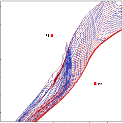
Flags for interpolated values
[1] The distance to one of the closer curves has been estimated as the one to the closest point in the curve [2] The distance to both the closest curves has been estimated as the one to the closest point in each curve [3] Only a range of values can be estimated [4] The point lies outside the area covered by the isochrones [5] No estimation has been posible
Example
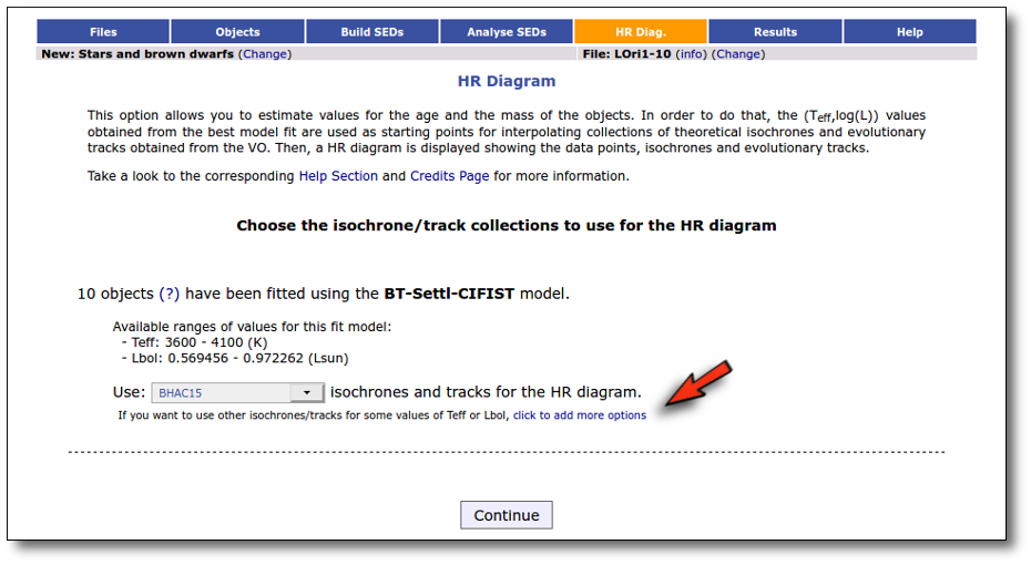
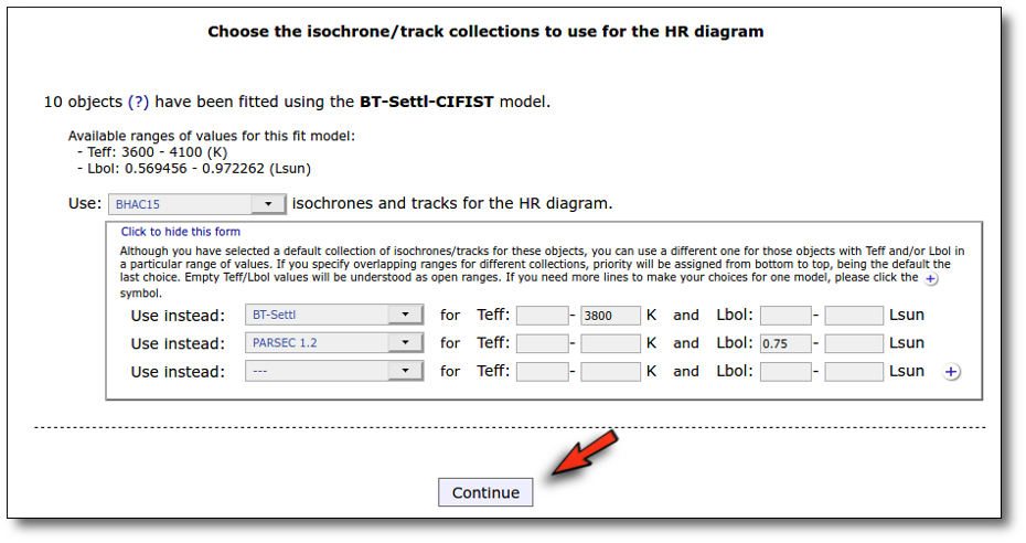
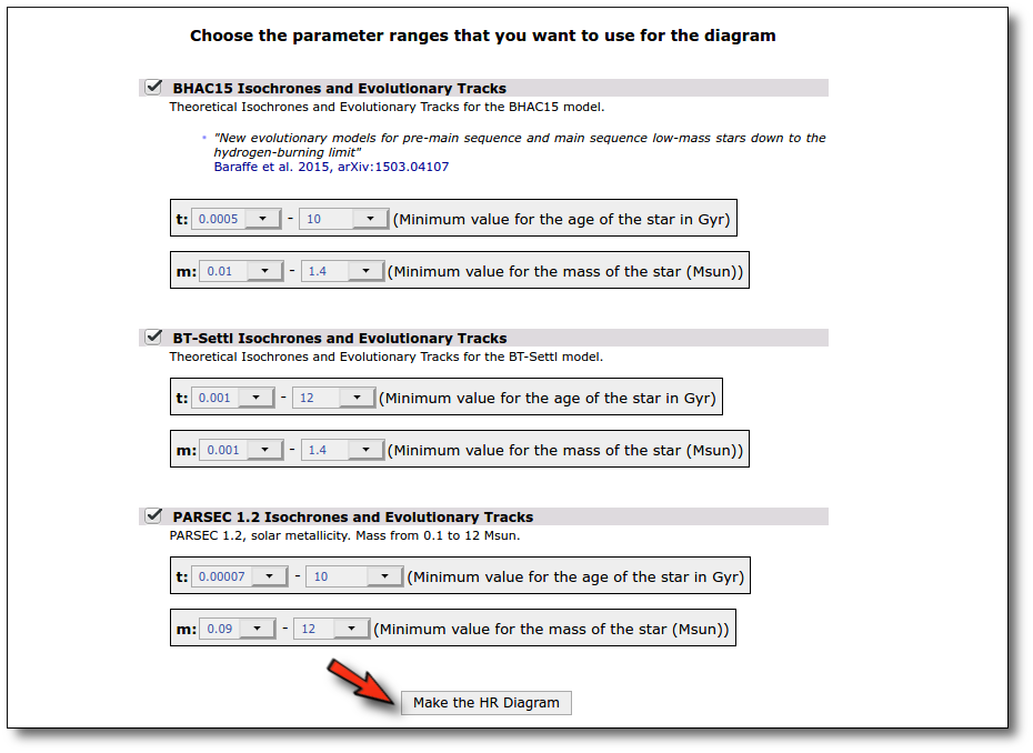
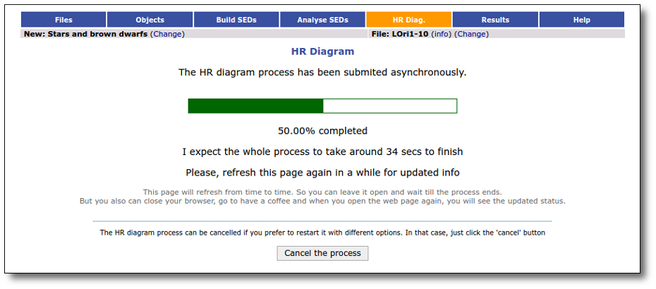

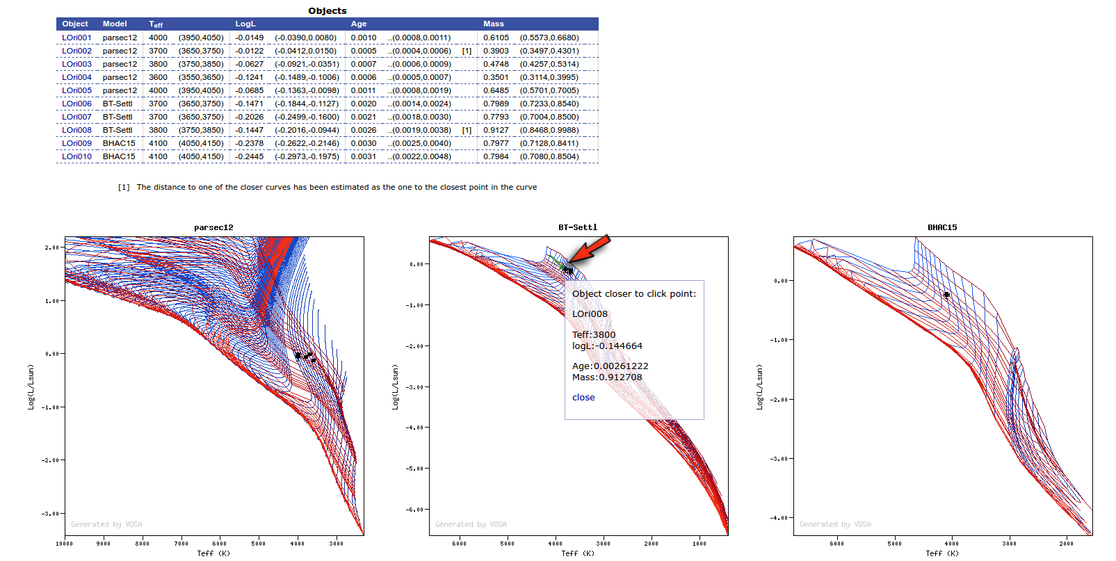
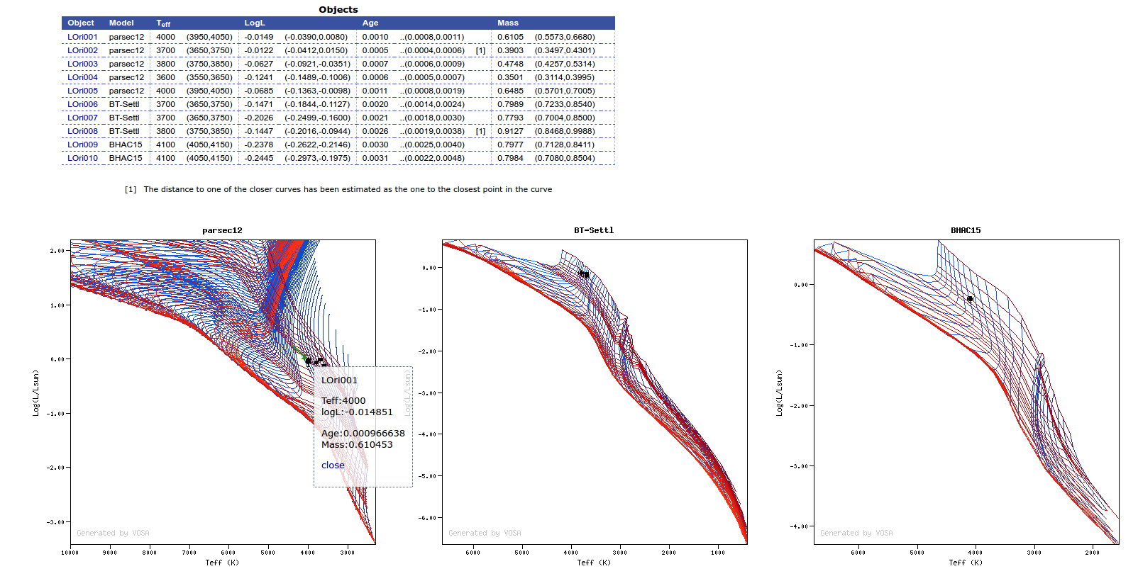
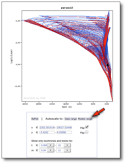
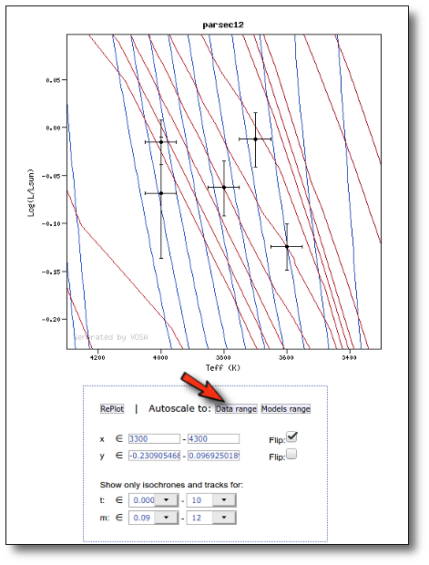
Upper Limits
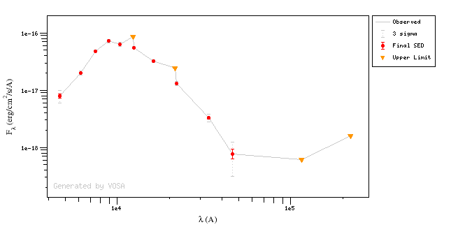
Statistics
Definitions
Definitions for a grouped distribution
In other words, the Percentile $P_k$ is defined as the value so that k/100 of the values in the distribution are smaller than it.
Normality tests
Save results
Download results
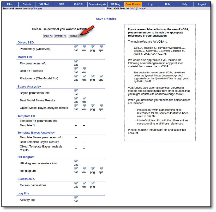
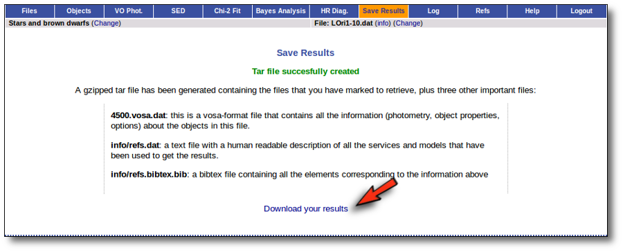
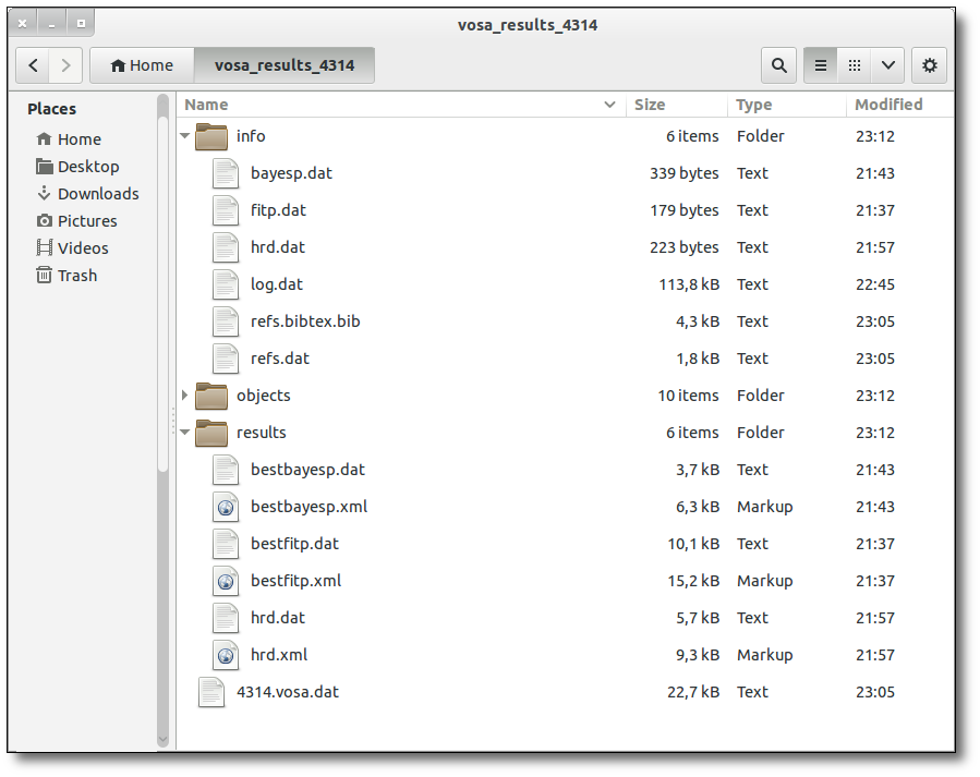
SAMP: Send results to other VO tools
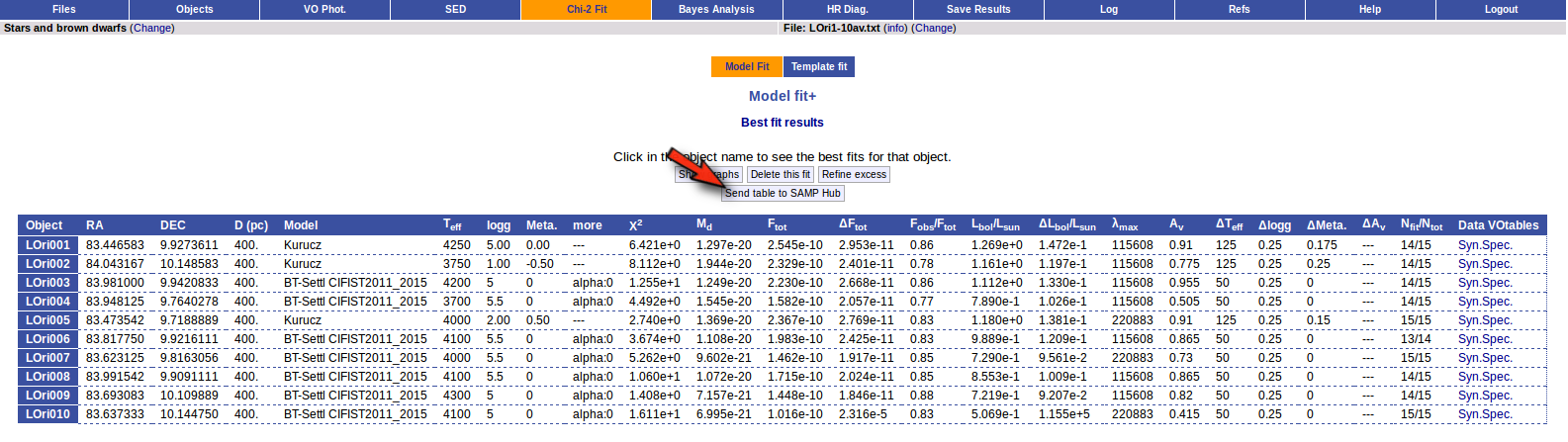
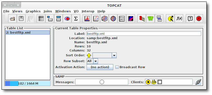
References
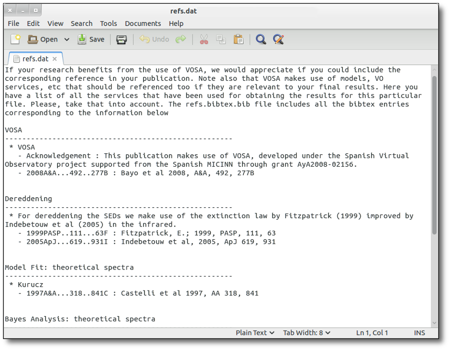
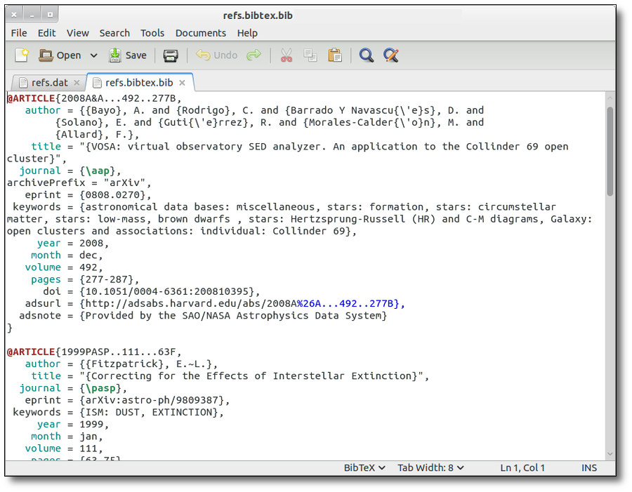
Log file
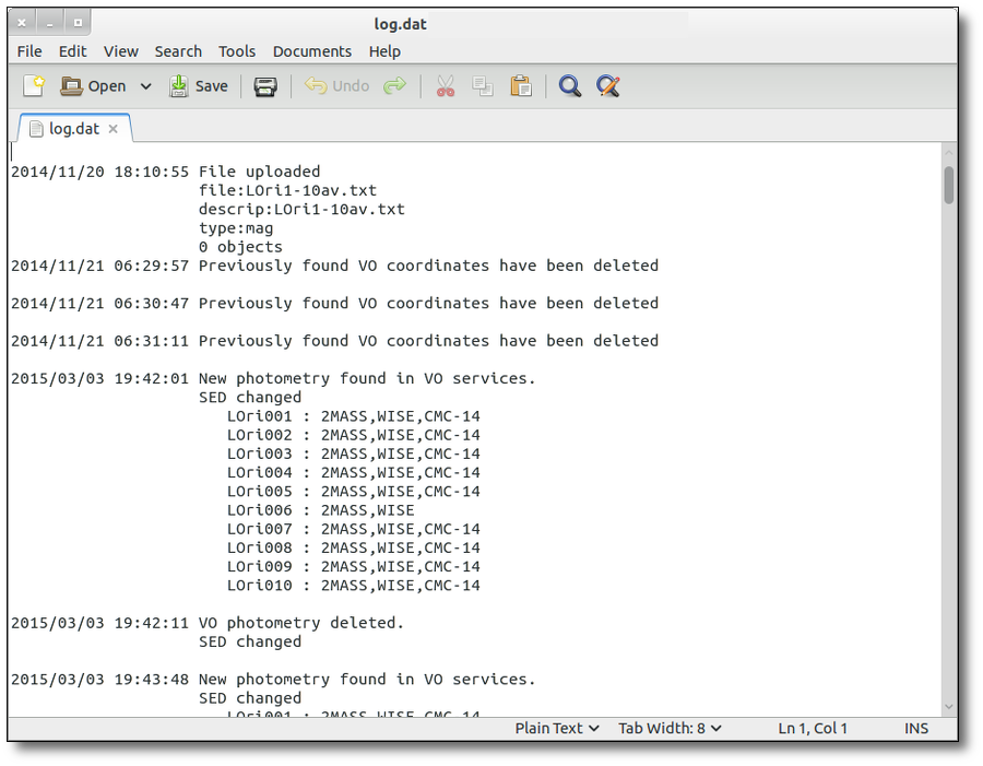
Plots
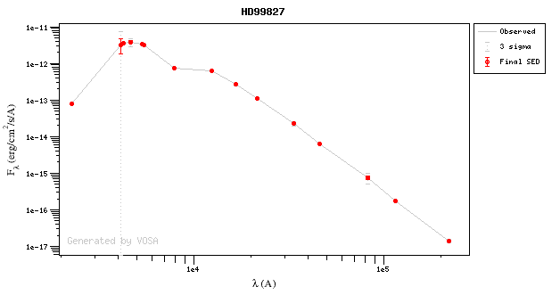
Graphs in Grace format
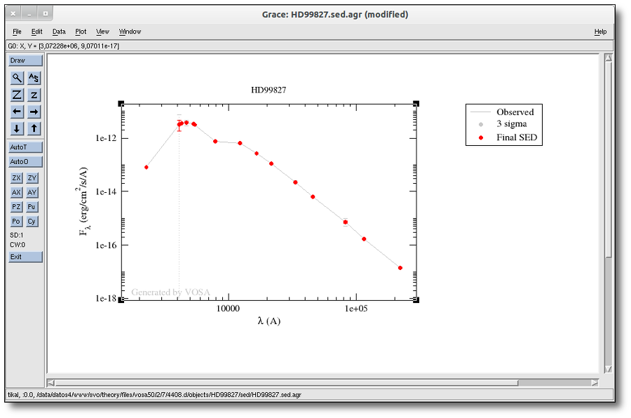
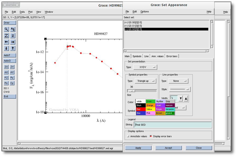
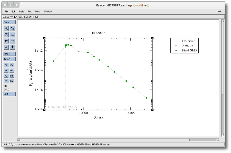
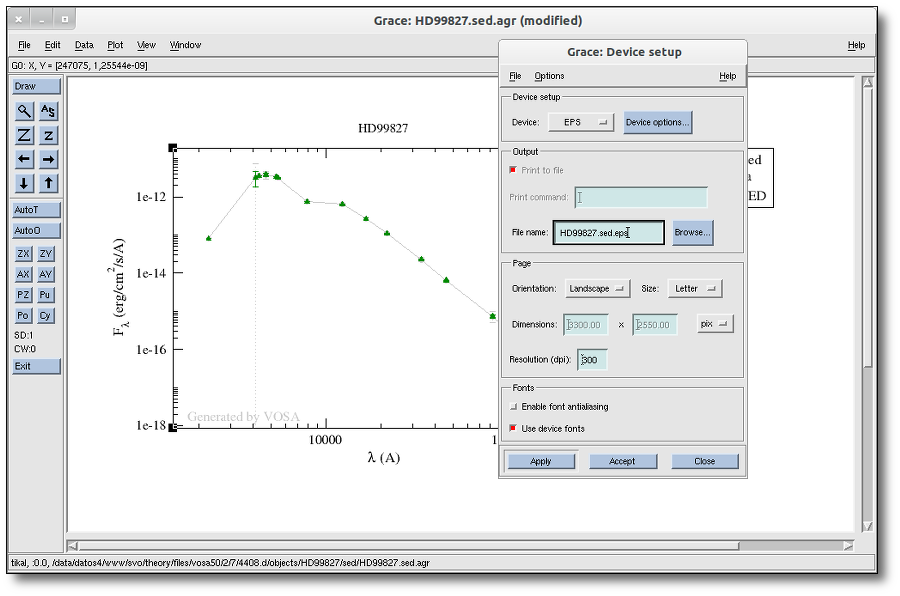
VOSA Architecture
Distributed environment.
Parallelized computing.
Asynchronous procedures.
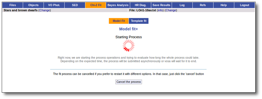
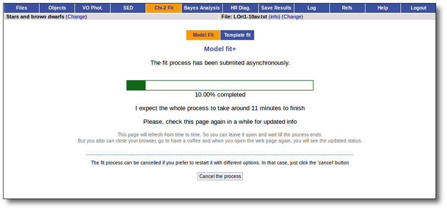
SVO Theoretical data server.
VO services.
SAMP.
Web design: pagination
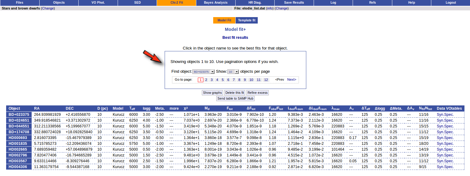
Phys. Constants
FAQ
Distances
Catalogs / Photometry
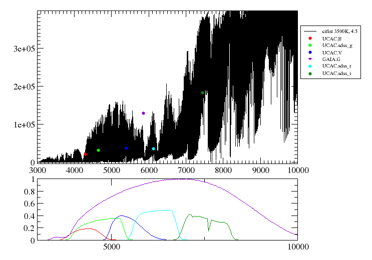
Model fit
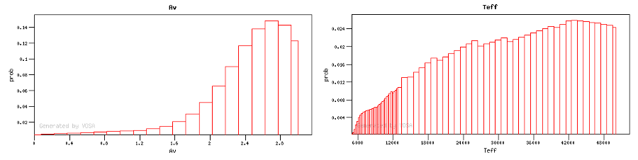
Output products
Use Case: From SED fitting to Age estimation. The case of Collinder 69
Introduction
Formating user data
Object
RA(deg)
DEC(deg)
Distance (pc)
Av
LOri001 83.446583 9.9273611 400 0.36209598 LOri002 84.043167 10.148583 400 0.36209598
Object
CFHT (R)
CFHT (I)
IRAC (I1)
IRAC (I2)
IRAC (I3)
IRAC (I4)
LOri001
13.21 12.52
10.228±0.003 10.255±0.004 10.214±0.009 10.206±0.01 LOri002
13.44 12.64
9.935±0.003 10.042±0.003 9.93±0.009 9.88±0.008

Uploading a user file.

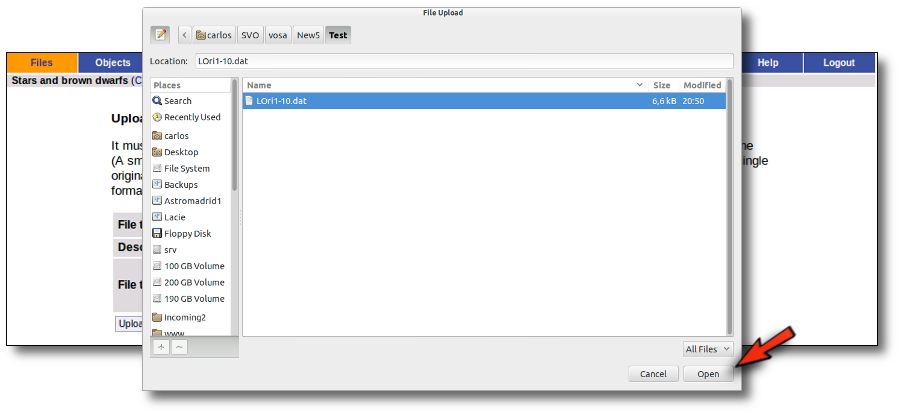
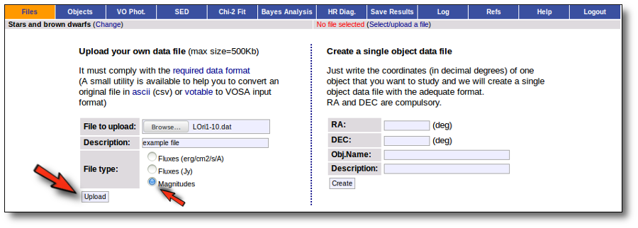
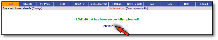
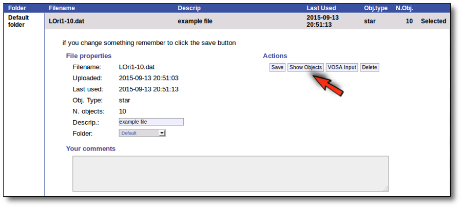
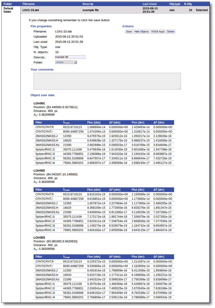
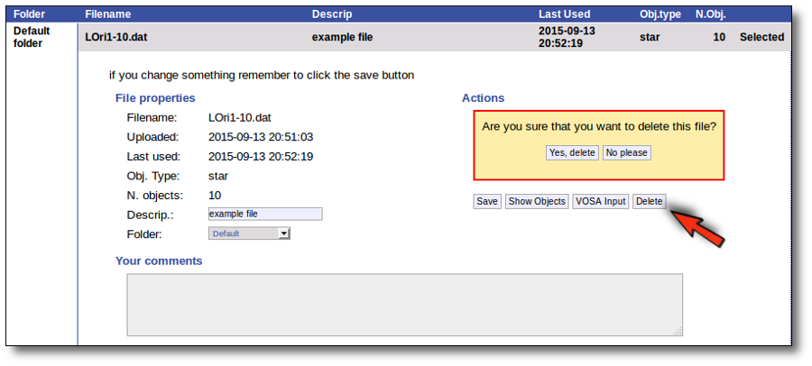
Obtaining photometry from the VO.
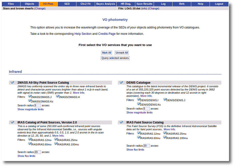
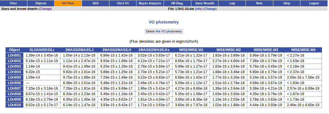
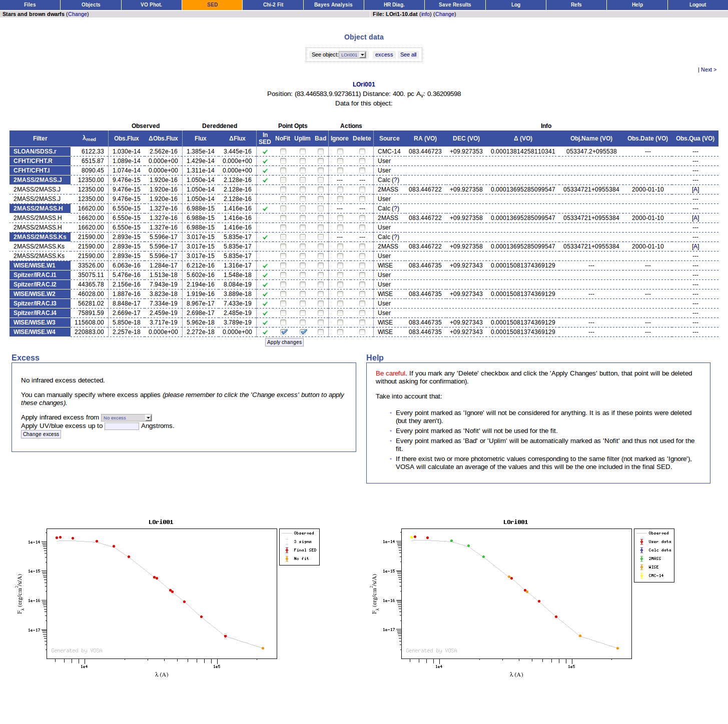
Model fit.
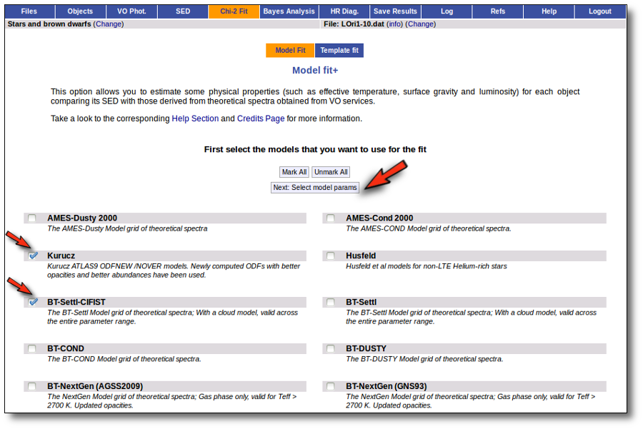
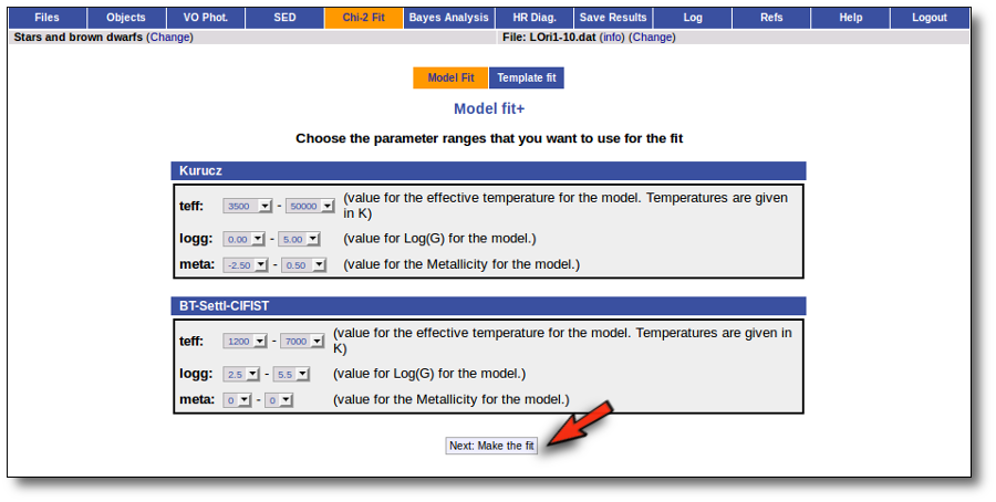
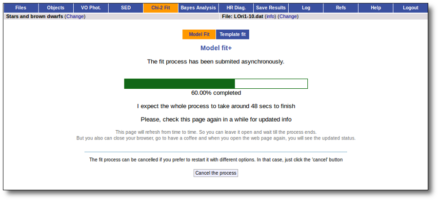
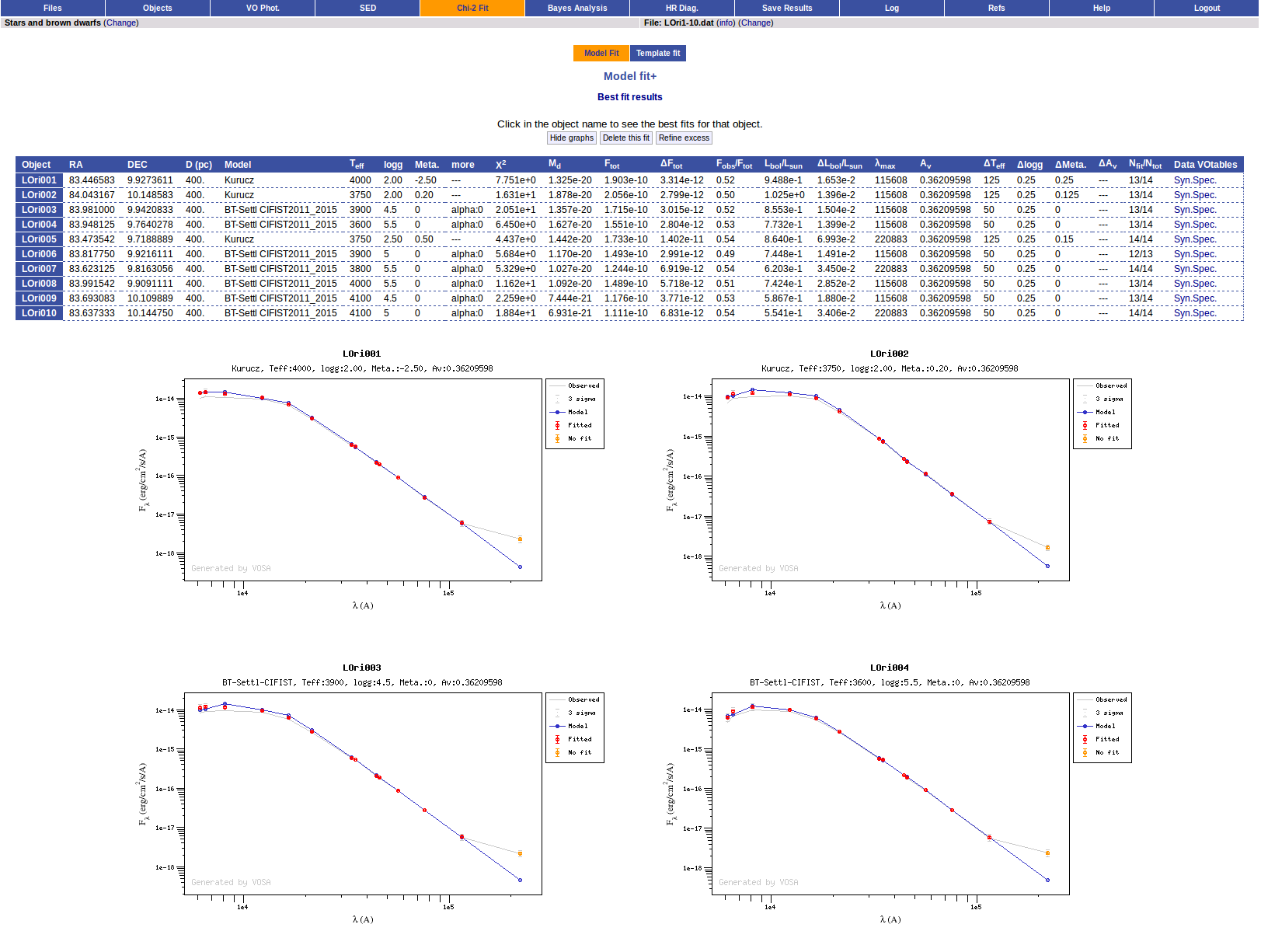
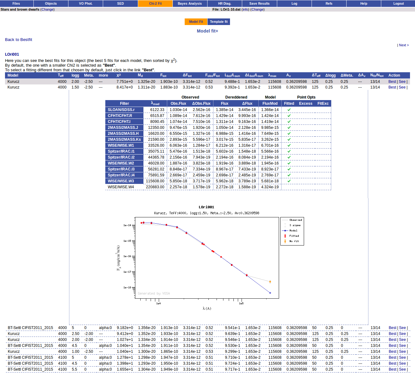
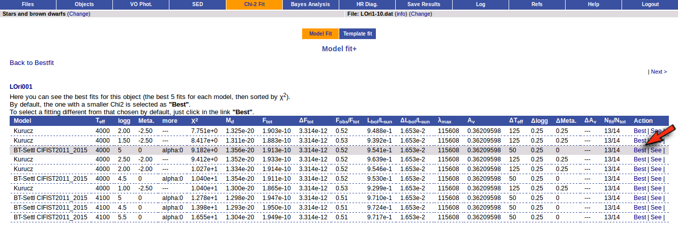
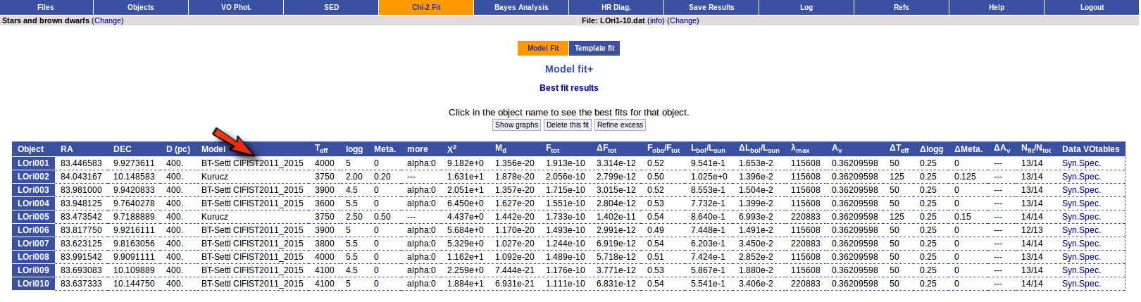
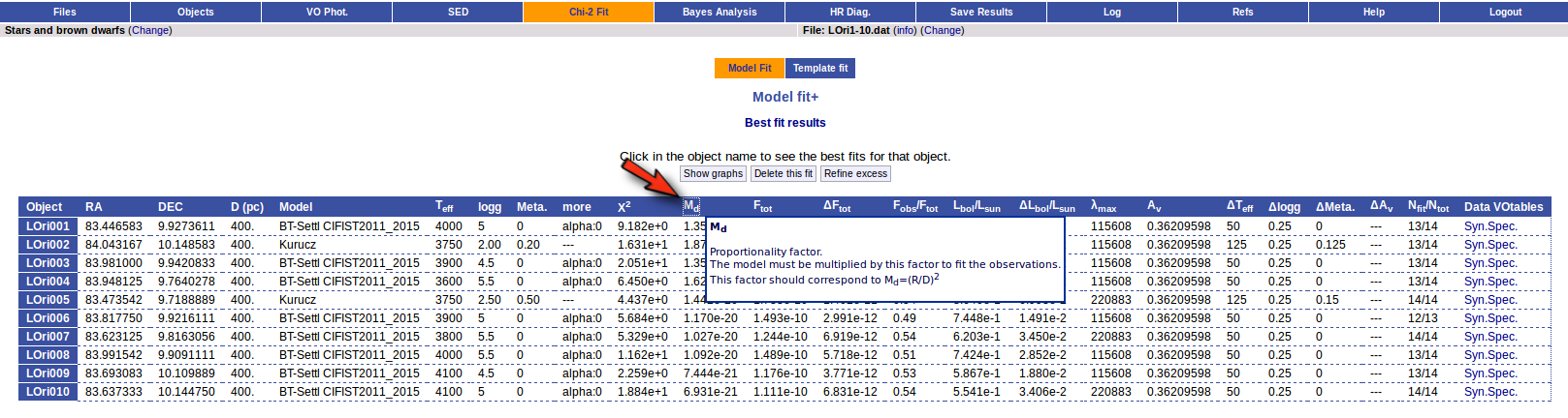
Object
Teff
Log(G)
Meta.
Ftot
Lbol/Lsun
LOri001 4000 5.0 0.0 1.913e-10 ± 3.314e-12 0.9541 ± 0.01653 LOri002 3750 2.0 0.2 2.056e-10 ± 2.799e-12 1.025 ± 0.01396 LOri003 3900 4.5 0.0 1.715e-10 ± 3.015e-12 0.8553 ± 0.01504 LOri004 3600 5.5 0.0 1.551e-10 ± 2.804e-12 0.7732 ± 0.01399 LOri005 3750 2.5 0.5 1.733e-10 ± 1.402e-11 0.864 ± 0.06993 LOri006 3900 5.0 0.0 1.493e-10 ± 2.991e-12 0.7448 ± 0.01491 LOri007 3800 5.5 0.0 1.244e-10 ± 6.919e-12 0.6203 ± 0.0345 LOri008 4000 5.5 0.0 1.489e-10 ± 5.718e-12 0.7424 ± 0.02852 LOri009 4100 4.5 0.0 1.176e-10 ± 3.771e-12 0.5867 ± 0.0188 LOri010 4100 5.0 0.0 1.111e-10 ± 6.831e-12 0.5541 ± 0.03406 Bayesian analysis.
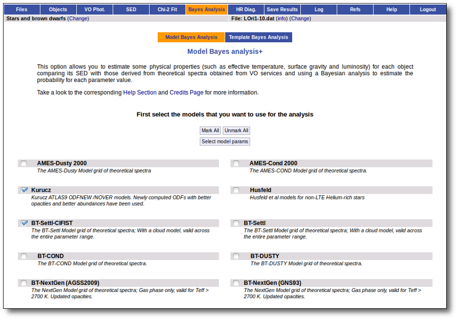
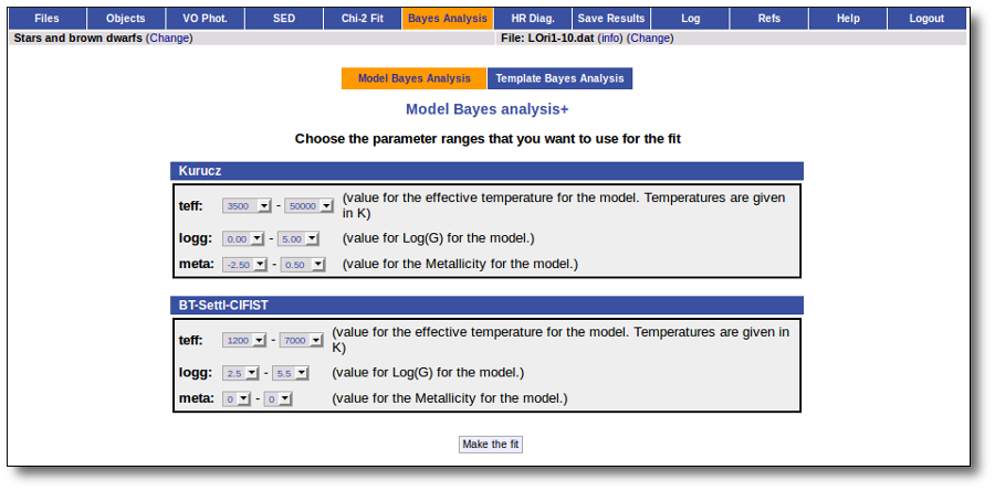
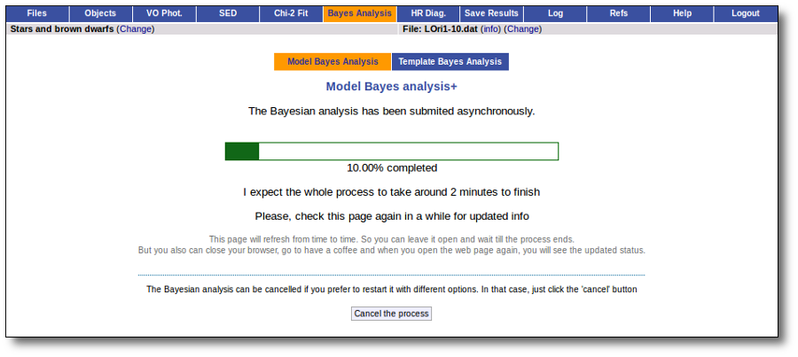
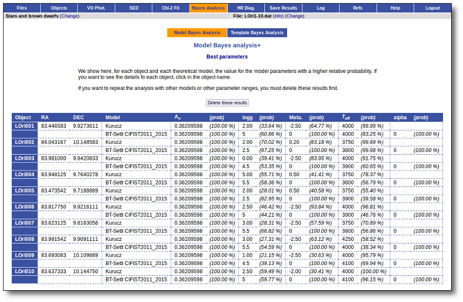
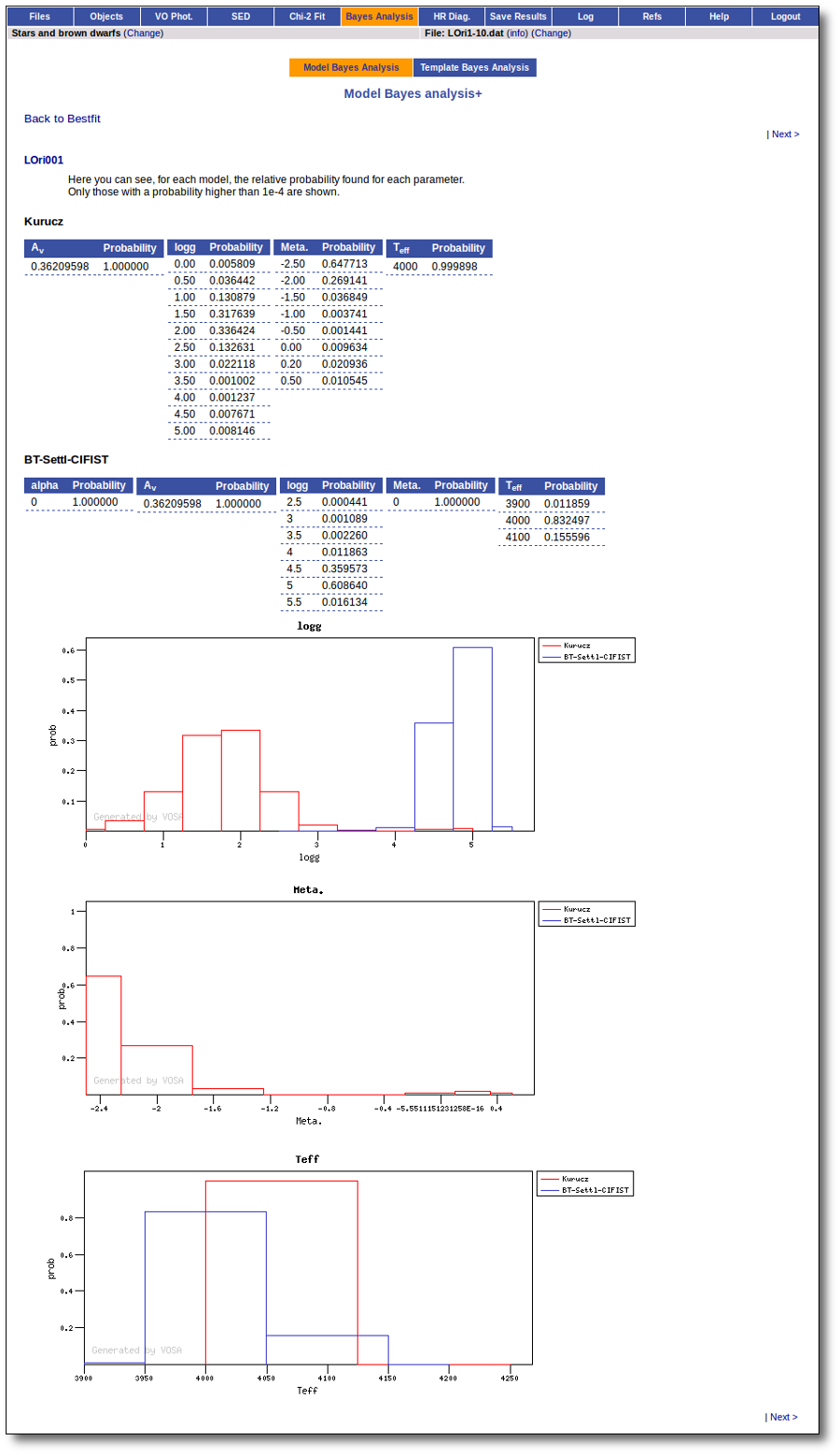
HR diagram.
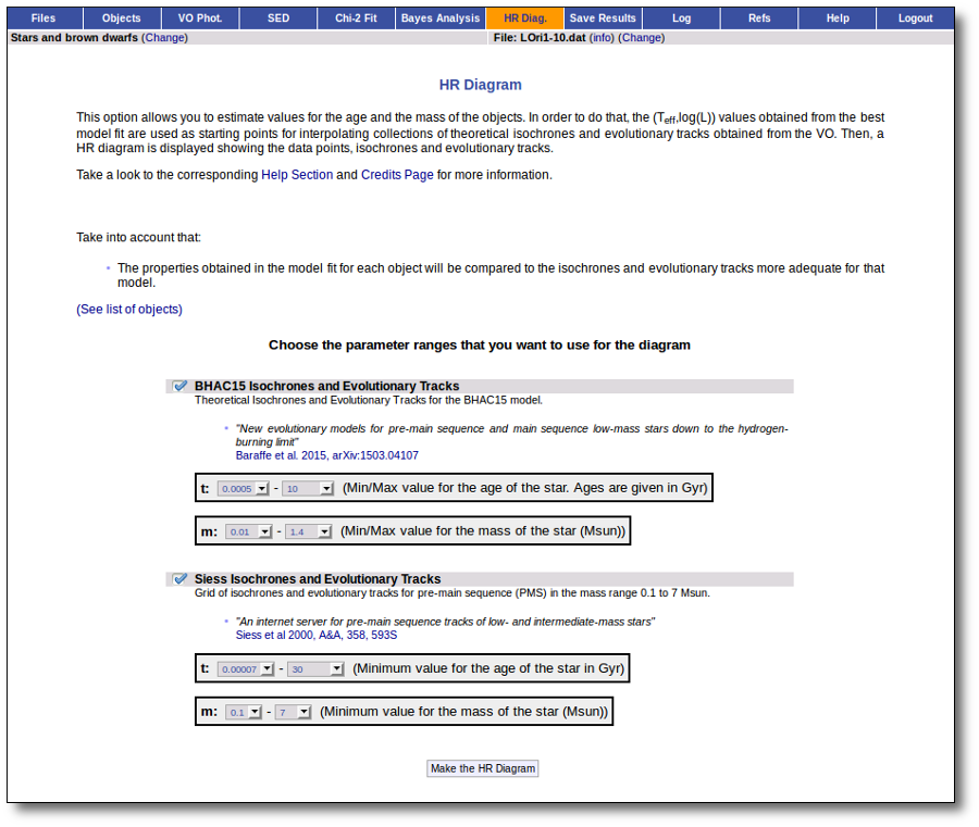
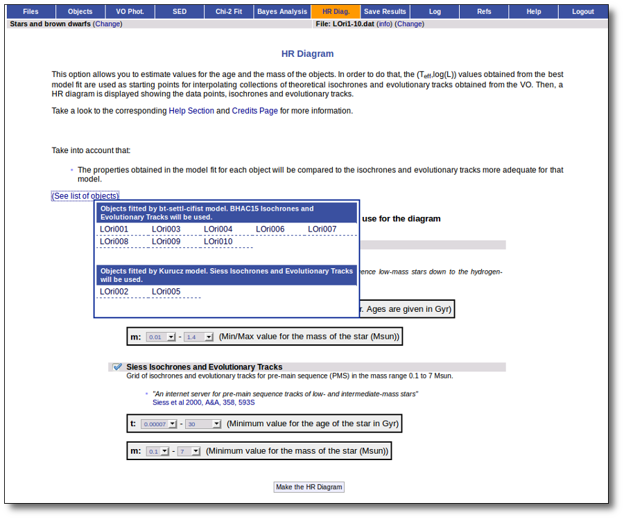

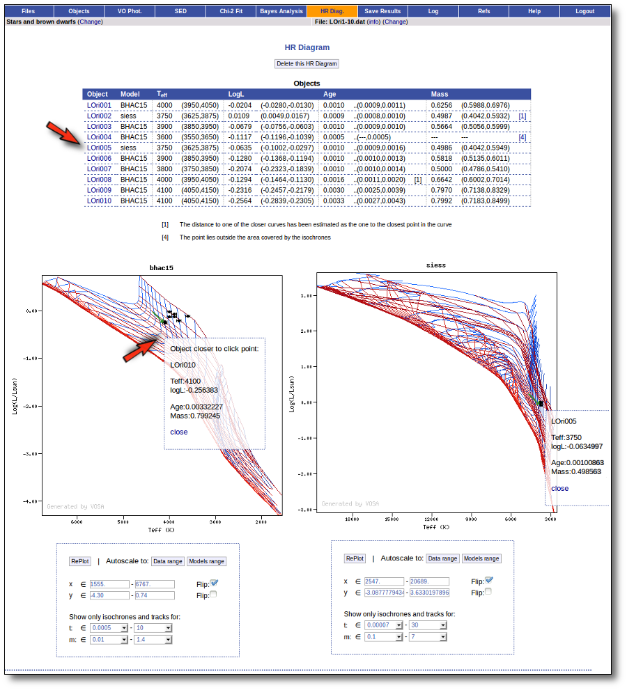
Object
Teff
Log(G)
Meta.
Ftot
Lbol/Lsun
Age (Gyr)
Mass/Msun
LOri001 4000 5.0 0.0 1.913e-10 ± 3.314e-12 0.9541 ± 0.01653 0.0009 - 0.0011 0.5988 - 0.6976 LOri002 3750 2.0 0.2 2.056e-10 ± 2.799e-12 1.025 ± 0.01396 0.0008 - 0.0010 0.4042 - 0.5932 LOri003 3900 4.5 0.0 1.715e-10 ± 3.015e-12 0.8553 ± 0.01504 0.0009 - 0.0010 0.5056 - 0.5999 LOri004 3600 5.5 0.0 1.551e-10 ± 2.804e-12 0.7732 ± 0.01399 ? - 0.0005 ? LOri005 3750 2.5 0.5 1.733e-10 ± 1.402e-11 0.864 ± 0.06993 0.0009 - 0.0016 0.4042 - 0.5949 LOri006 3900 5.0 0.0 1.493e-10 ± 2.991e-12 0.7448 ± 0.01491 0.0010 - 0.0013 0.5135 - 0.6011 LOri007 3800 5.5 0.0 1.244e-10 ± 6.919e-12 0.6203 ± 0.0345 0.0010 - 0.0014 0.4786 - 0.5410 LOri008 4000 5.5 0.0 1.489e-10 ± 5.718e-12 0.7424 ± 0.02852 0.0011 - 0.0020 0.6002 - 0.7014 LOri009 4100 4.5 0.0 1.176e-10 ± 3.771e-12 0.5867 ± 0.0188 0.0025 - 0.0039 0.7138 - 0.8329 LOri010 4100 5.0 0.0 1.111e-10 ± 6.831e-12 0.5541 ± 0.03406 0.0027 - 0.0043 0.7183 - 0.8499 Save Results.
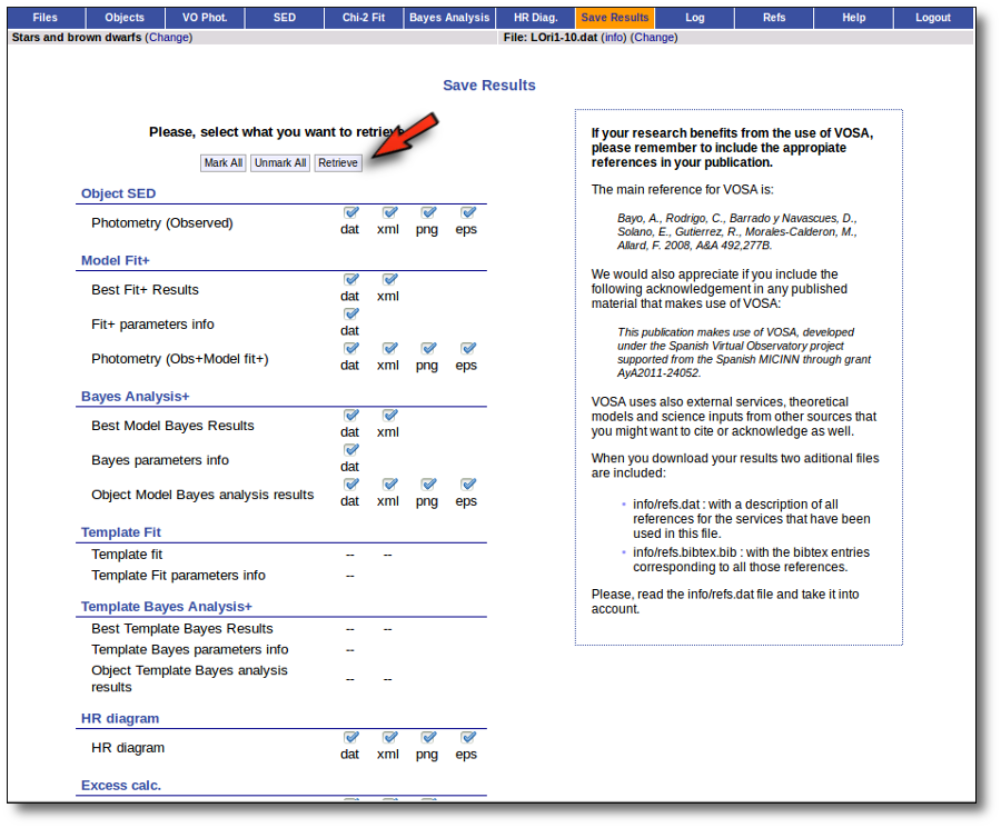

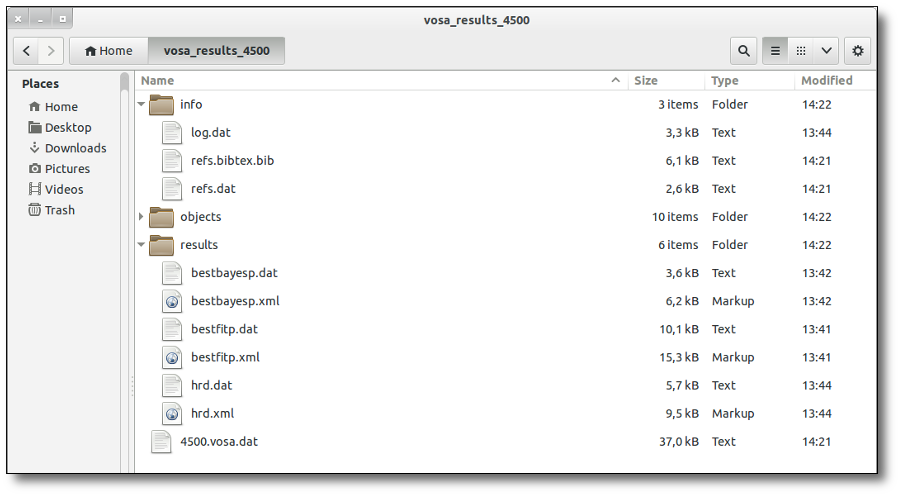
Quality assessment tests
Quality: Stellar libraries tests
Elodie library
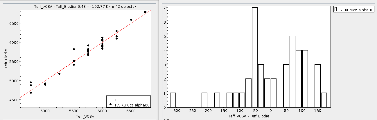
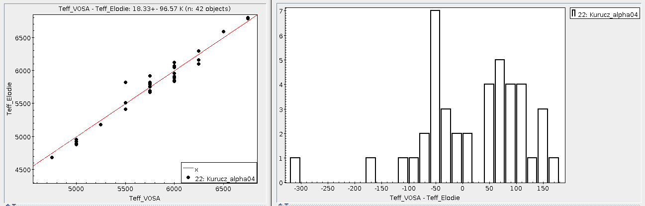
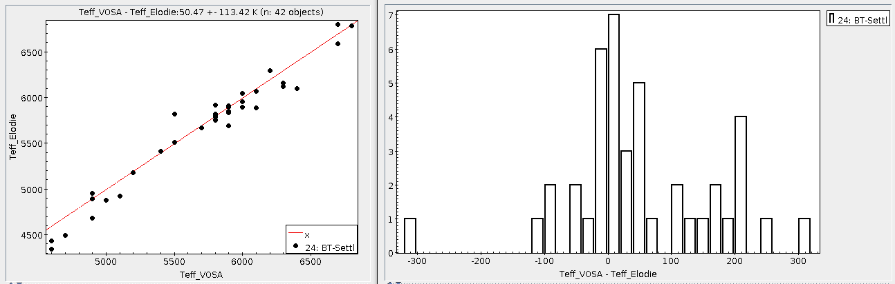
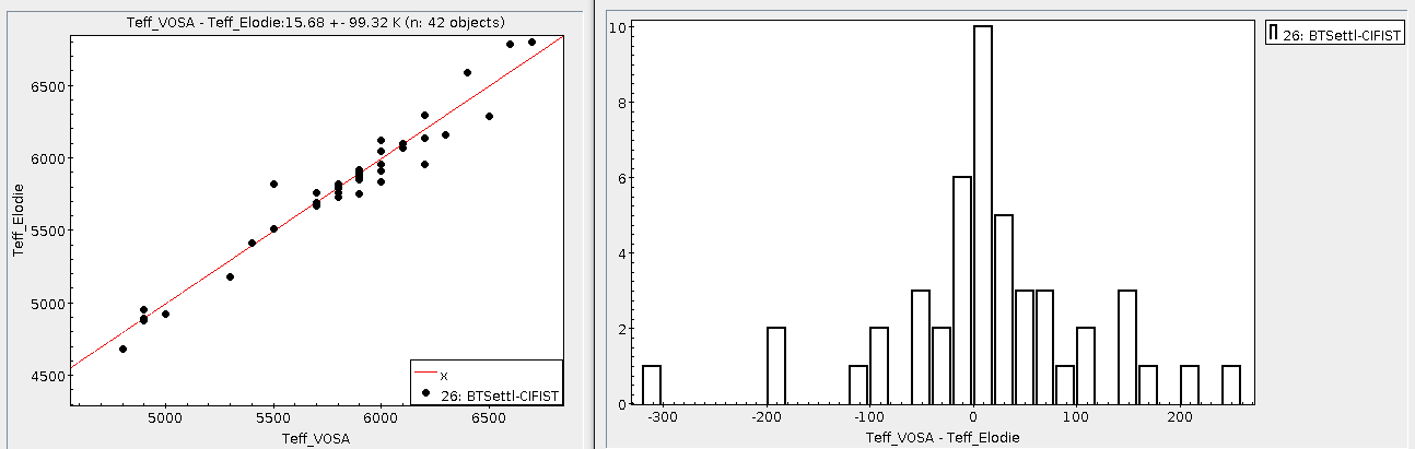
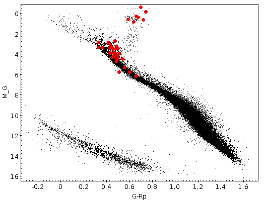
Object
RA (deg)
DEC (deg)
HD000693 2.81607 -15.46798 HD004307 11.36953 -12.88081 HD005015 13.26748 61.12397 HD009562 23.42848 -7.02534 HD017674 42.76785 30.28674 HD019476 47.37405 44.85754 HD029310 69.38328 15.14645 HD039587 88.59576 20.27617 HD043947 94.91739 16.01325 HD055575 108.95891 47.23996 HD059984 113.02401 -8.88133 HD061606 114.9972 -3.59751 HD064606 118.64241 -1.41225 HD073108 130.0534 64.32794 HD081809 141.94492 -6.07119 HD085503 148.1909 26.00695 HD089010 154.13454 23.5031 HD102224 176.51256 47.77941 HD104979 181.30225 8.73299 HD105755 182.56615 54.48815 HD107213 184.87302 28.15692 HD108954 187.7089 53.07661 HD128167 218.67007 29.74513 HD130322 221.88635 -0.28148 HD134083 226.82529 24.86919 HD134169 227.07524 3.93059 HD139798 234.5676 46.79775 HD141004 236.61089 7.35307 HD150177 249.91304 -9.55459 HD150997 250.72401 38.92225 HD159222 263.00415 34.27115 HD165401 271.40607 4.65717 HD165908 271.7564 30.56214 HD168009 273.88528 45.20932 HD186408 295.45398 50.52506 HD187123 296.74213 34.41952 HD188510 298.79034 10.74094 HD195633 308.09995 6.51757 HD199960 315.141 -4.73026 HD217014 344.36658 20.76883 HD219623 349.17627 53.21347 HD220954 351.99207 6.37899 VOSA and hot stars.
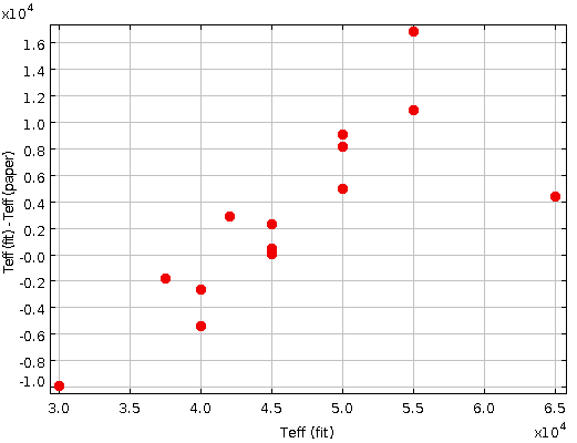
Object
Model
Teff (fit)
Teff (paper)
Teff(fit)-Teff(paper)
HE0001-2443 Husfeld 50000.0 40975.0 9025.0 HE0111-1526 Kurucz 42000.0 39152.0 2848.0 HE0342-1702 TLUSTY 50000.0 41914.0 8086.0 HE0914-0314 Husfeld 50000.0 45136.0 4864.0 HE0958-1151 Husfeld 55000.0 44125.0 10875.0 HE1047-0637 Husfeld 65000.0 60650.0 4350.0 HE1136-1641 TLUSTY 45000.0 44646.0 354.0 HE1203-1048 TLUSTY 40000.0 45439.0 -5439.0 HE1238-1745 Husfeld 55000.0 38219.0 16781.0 HE1258+0113 Husfeld 37500.0 39359.0 -1859.0 HE1310-2733 Kurucz 30000.0 40000.0 -10000.0 HE1316-1834 TLUSTY 45000.0 42811.0 2189.0 HE1446-1058 TLUSTY 45000.0 45000.0 0.0 HE1513-0432 TLUSTY 40000.0 42699.0 -2699.0 Comparison with Yee et al. (2017ApJ...836...77Y)
Effective temperatures
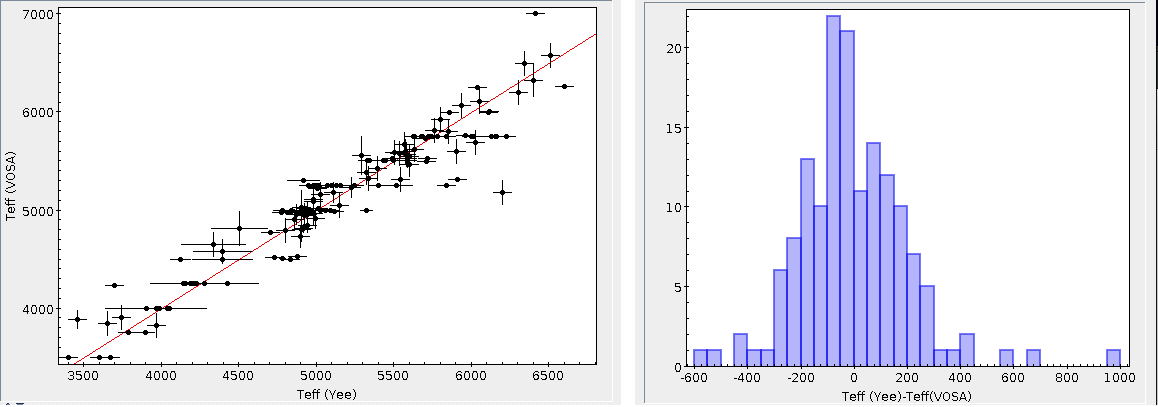
Surface gravities
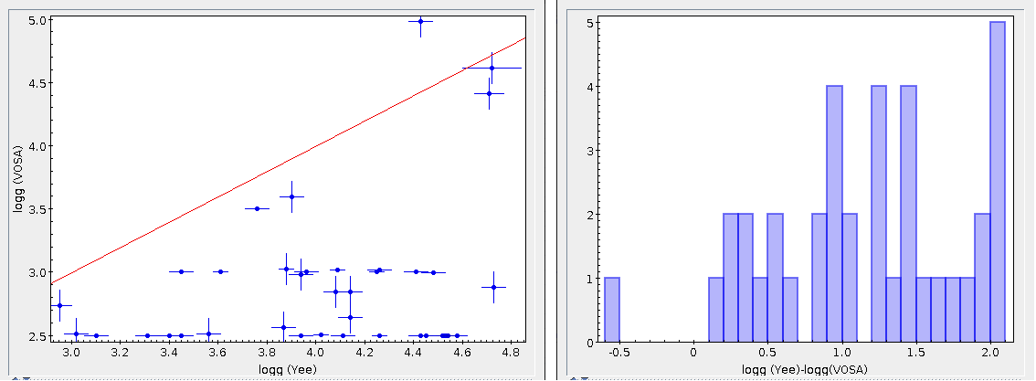
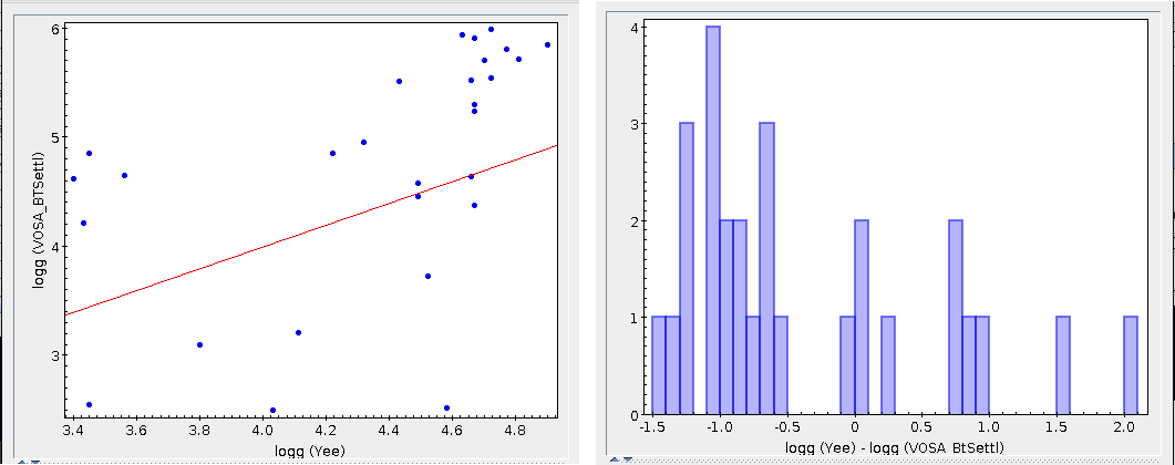
Metallicities
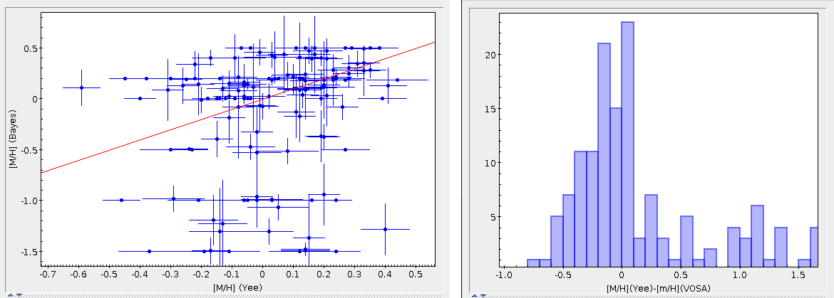
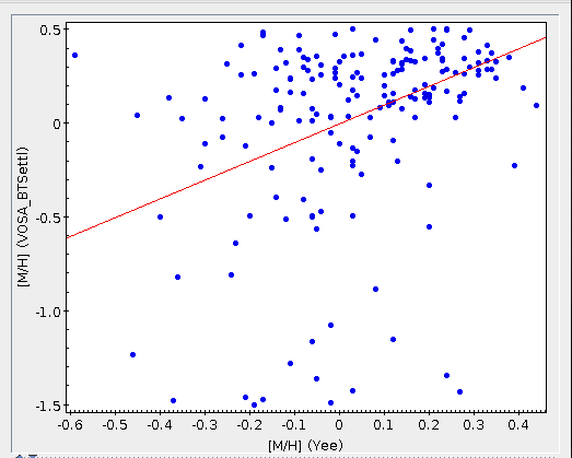
Radius
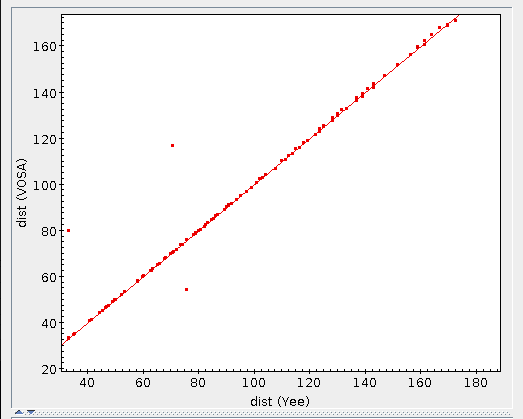
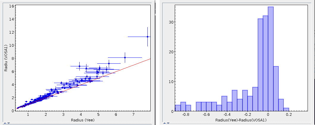
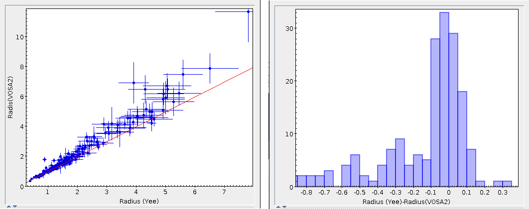
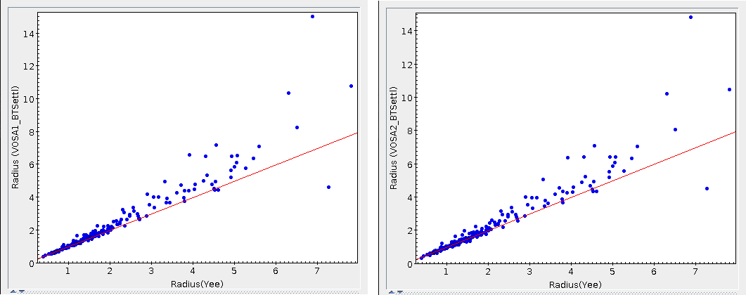
Masses
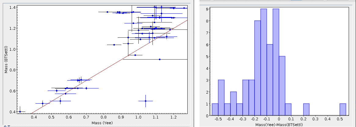
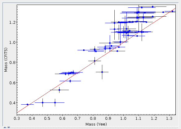
Comparison with Lindgren & Heiter 2017 (arXiv170508785L)
Summary
Sample and input parameters
Parameters determination
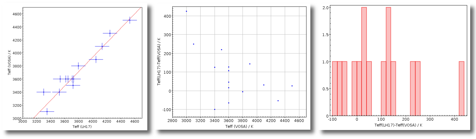
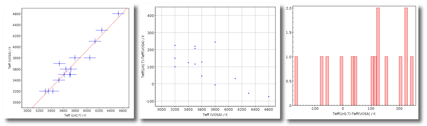
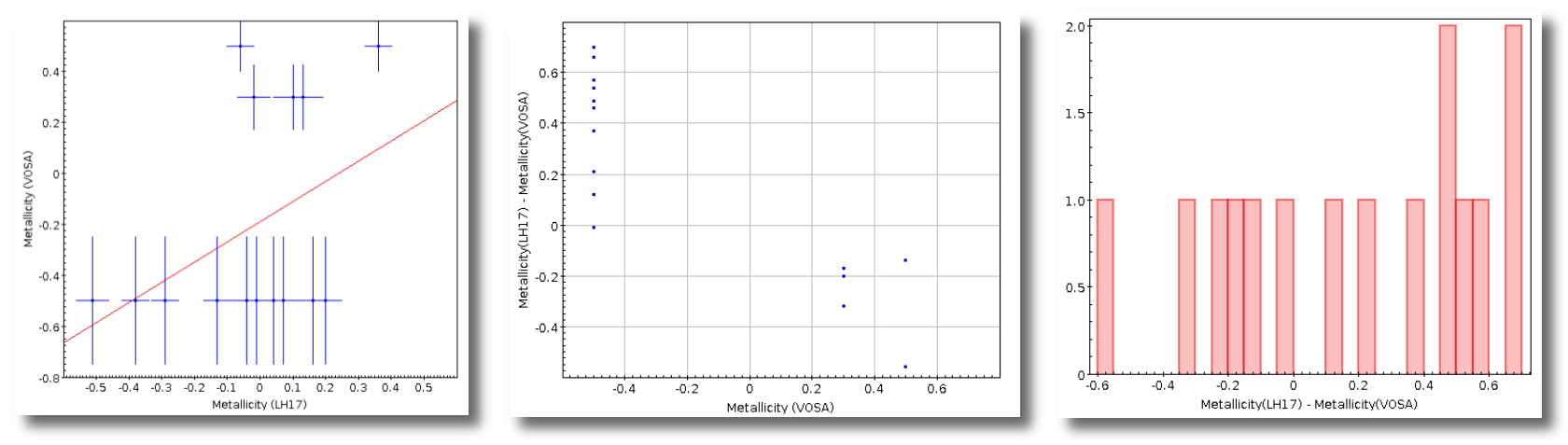
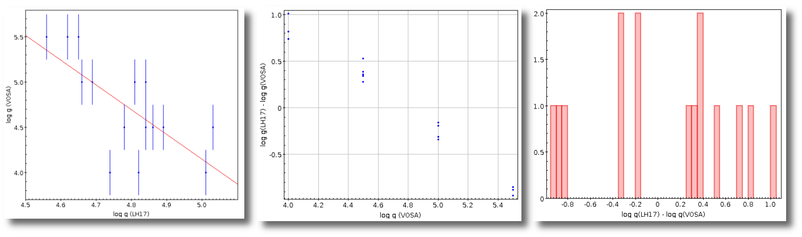

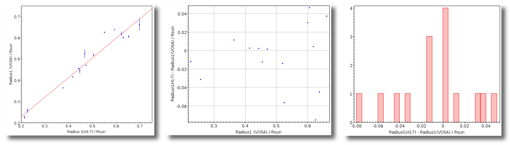
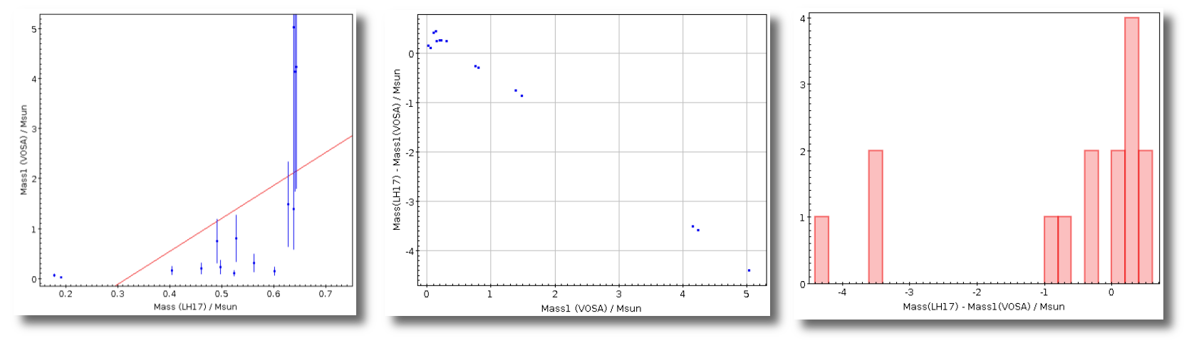
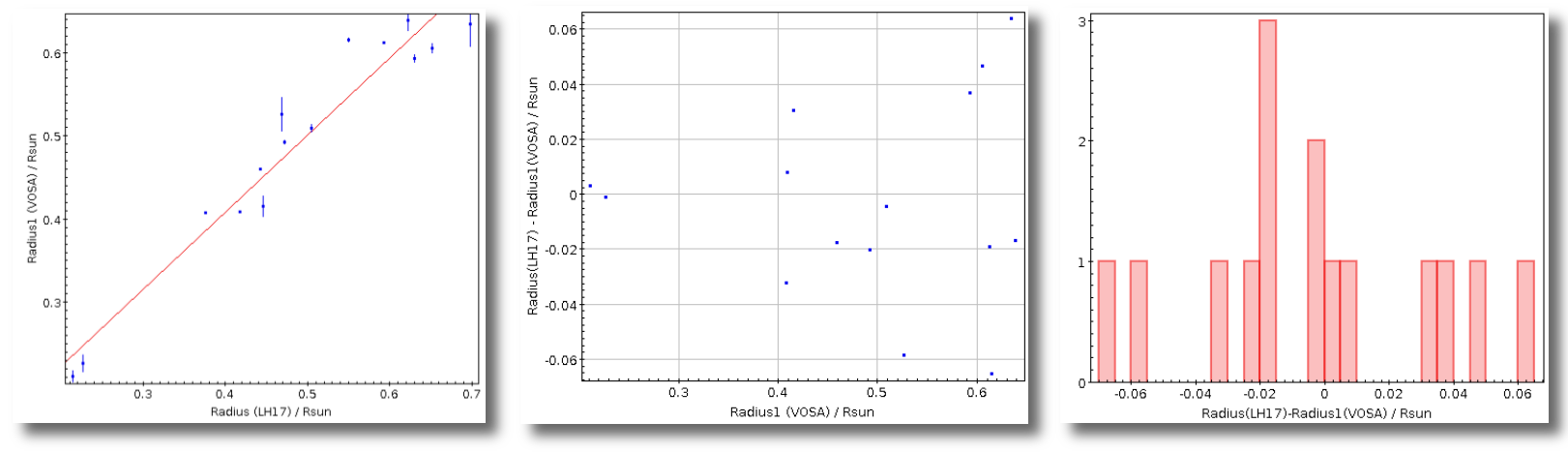
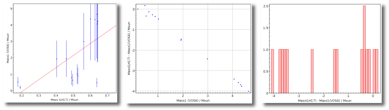
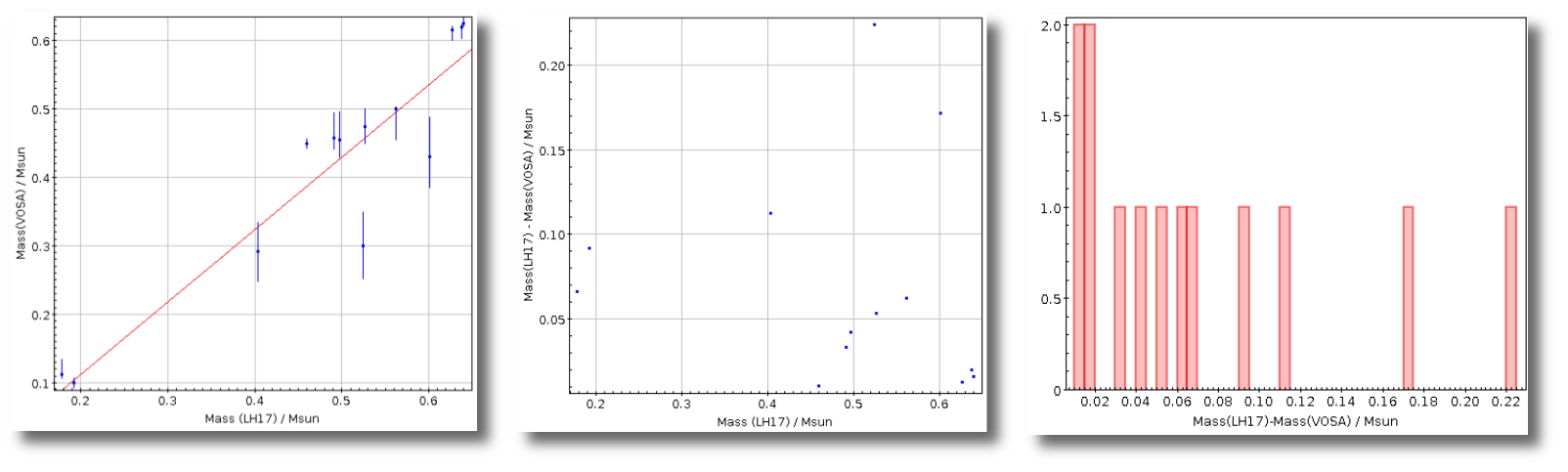
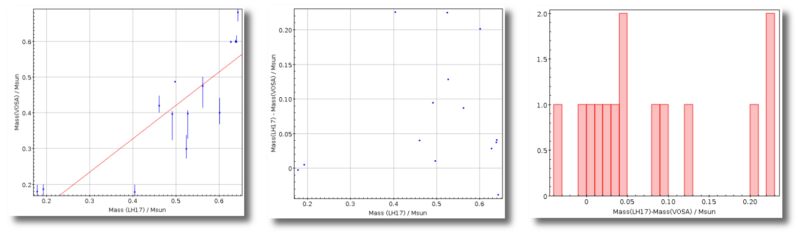
Comparison with 48-Carmencita stars
Summary
Sample and input parameters
Parameters determination
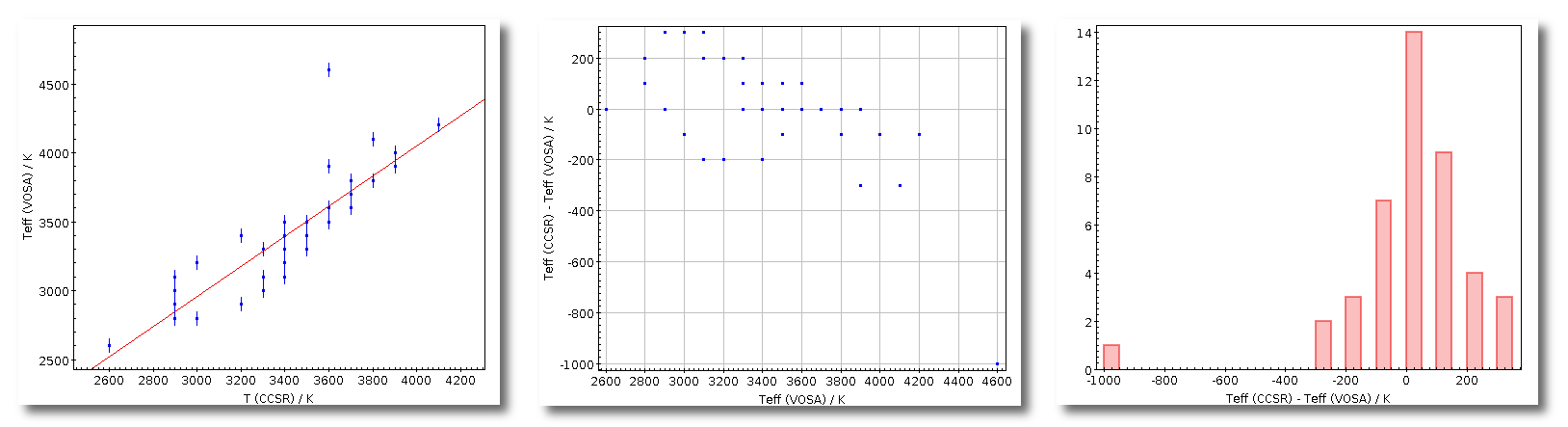

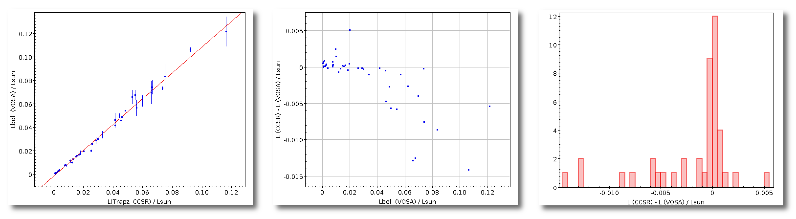
Comparison with Rajpurohit et al. 2017
Summary
Sample and input parameters
Parameters determination
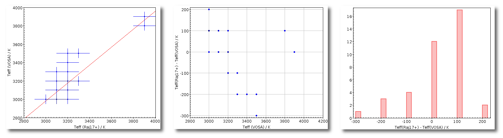
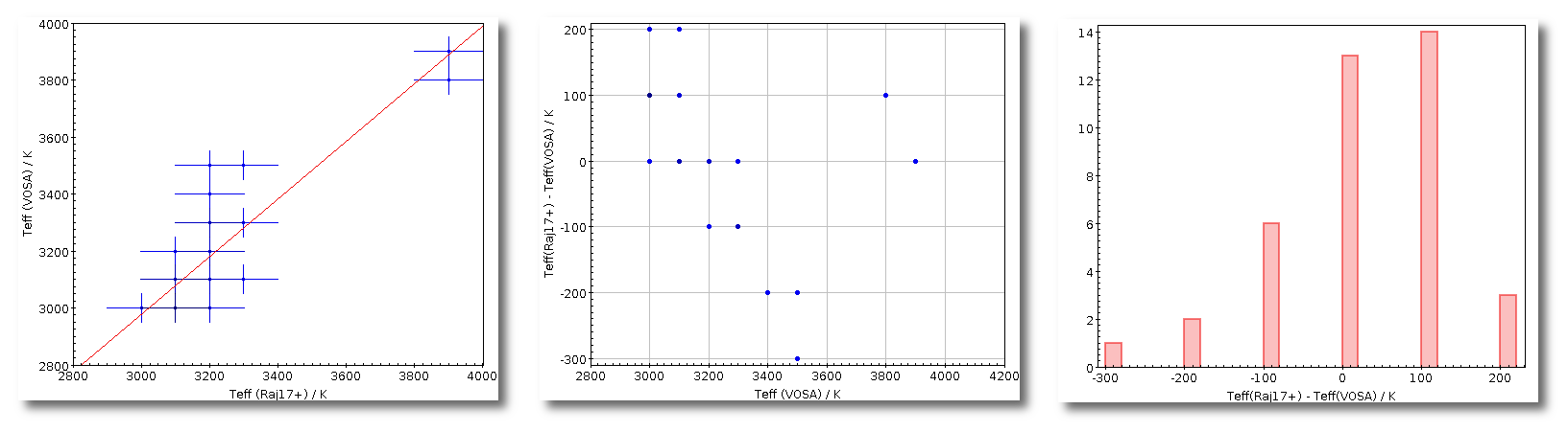
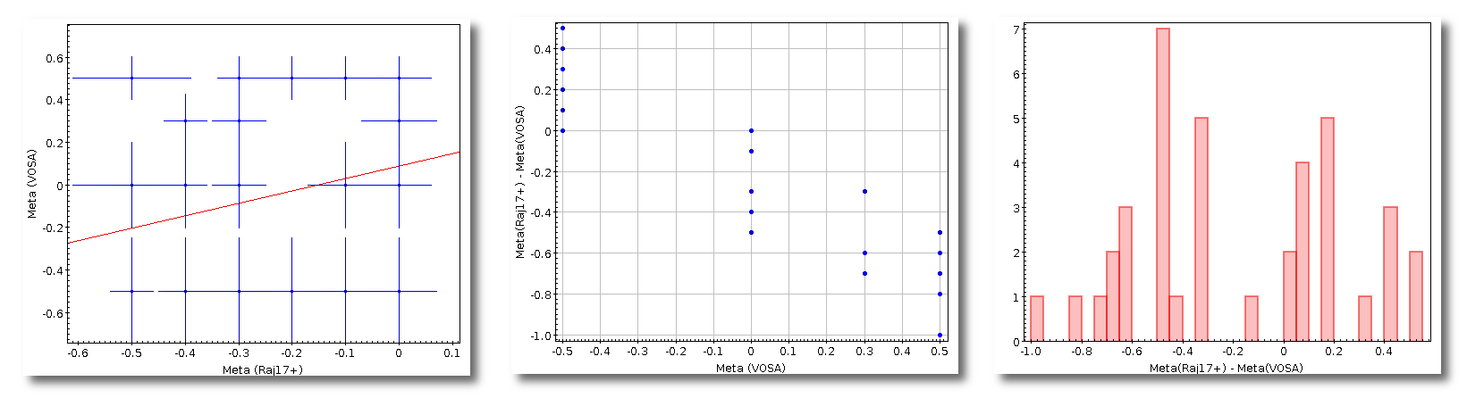
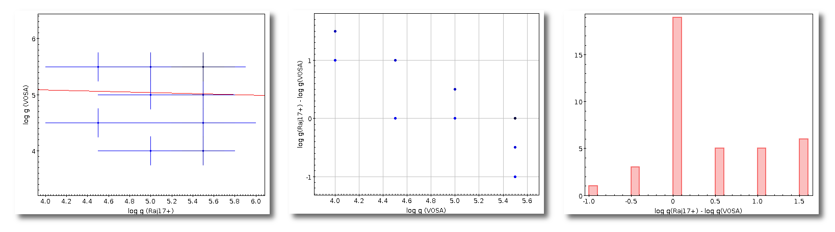
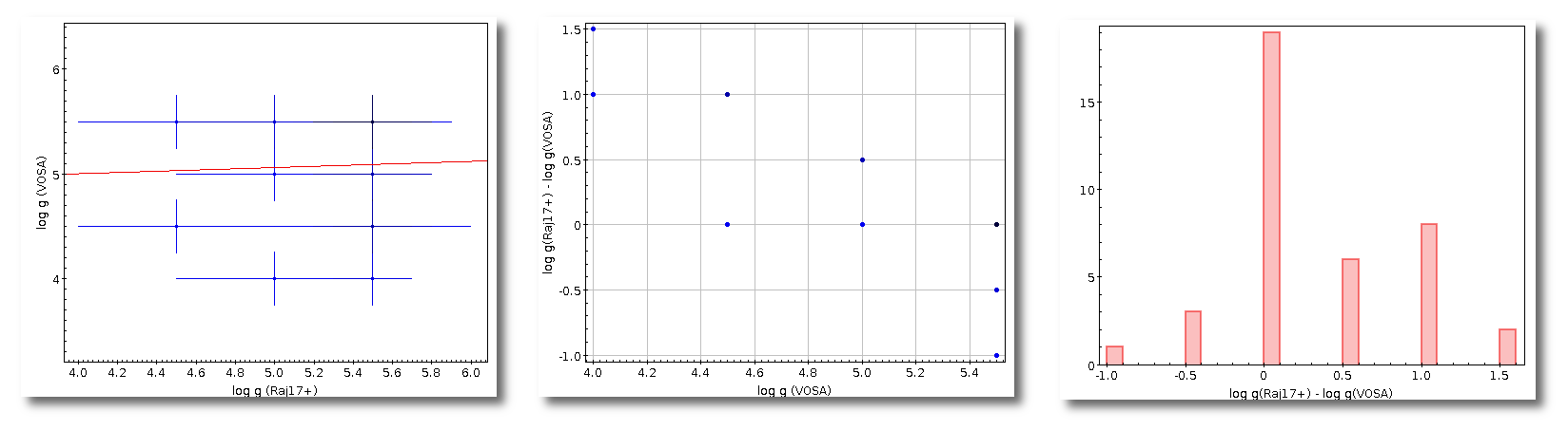
Quality: VO photometry tests
Flux comparison: APASS DR9 / Johnson (B,V bands)
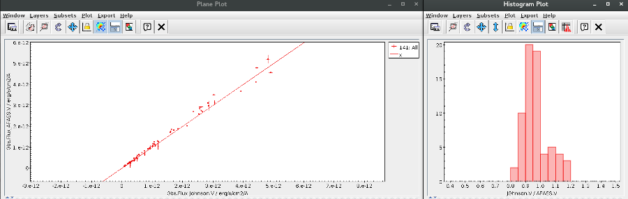
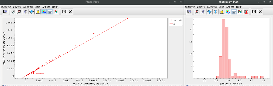
Flux comparison: SDSS DR12 / APASS DR9 (g,r,i bands)
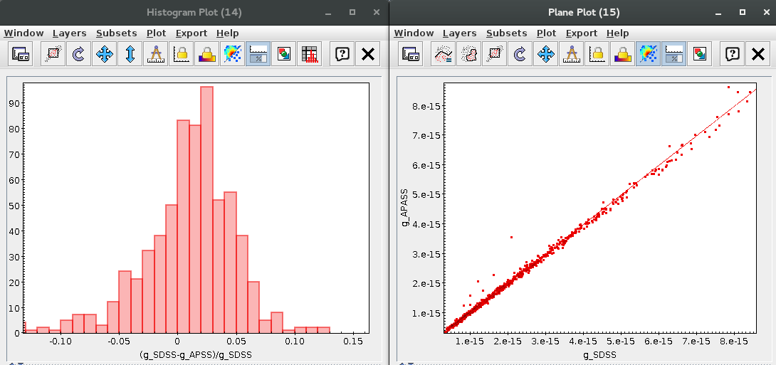
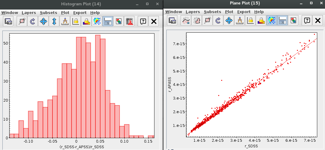
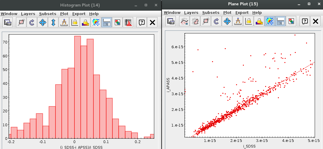
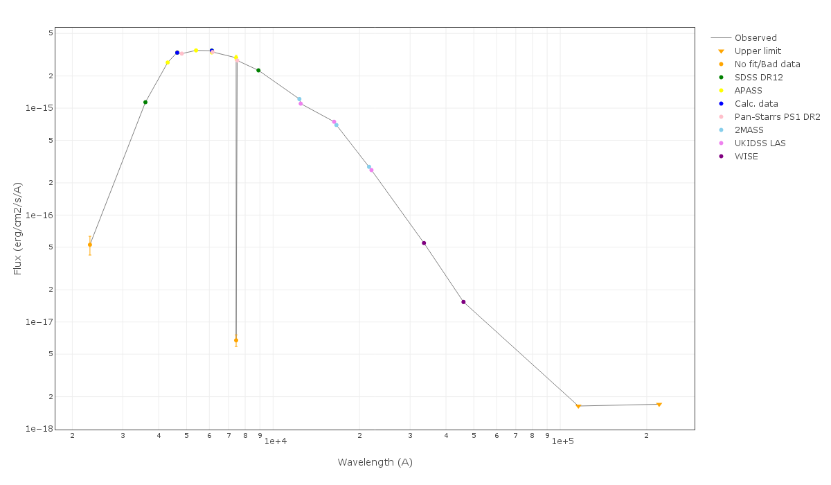
Flux comparison: SDSS DR9 / CTIO.DECam (g,r,z bands)
gmag<22.2 && rmag<22.2 && zmag<20.5 && e_gmag<0.2 && e_rmag<0.2 && e_zmag<0.2 && qmode && cl==6 && decam_anymask_1==0 && decam_anymask_2==0 && decam_anymask_3==0 && decam_anymask_4==0 && decam_anymask_5==0 && g<24.7 && r<23.9 && z<23
band
g
r
z
Median (SDSS/VPHAS+)
0.957
0.973
1.024
Q10 (SDSS/VPHAS+)
0.861
0.882
0.959
Q90 (SDSS/VPHAS+)
1.017
1.018
1.083
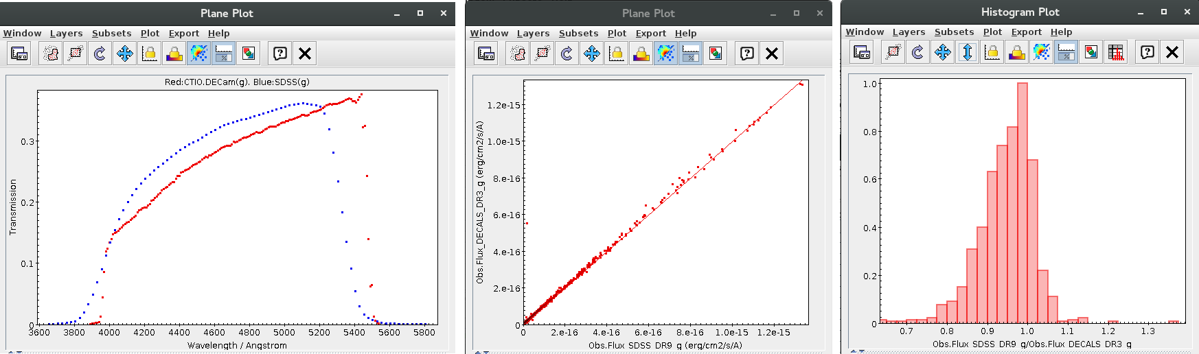
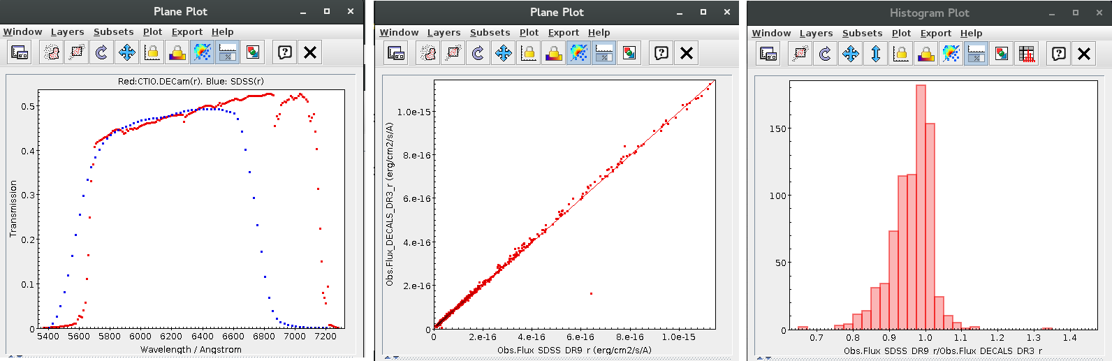
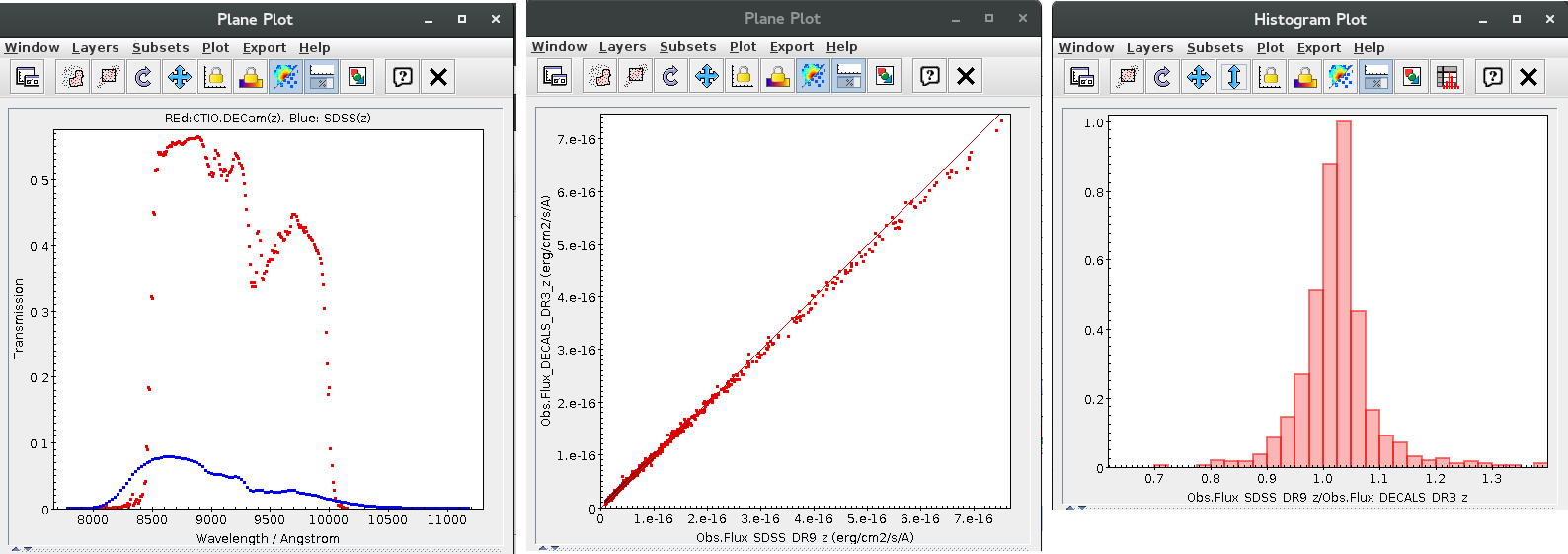
Flux comparison SDSS DR9 / IPHAS DR2 (r,i bands)
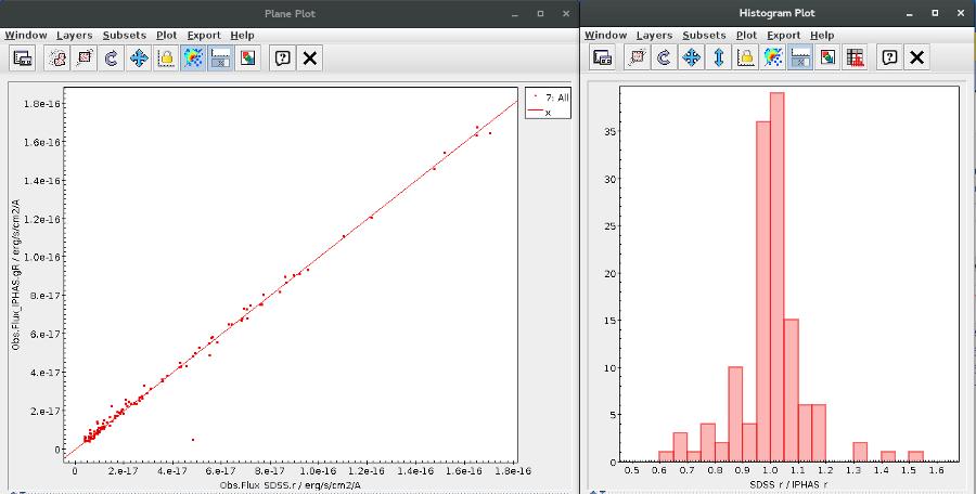
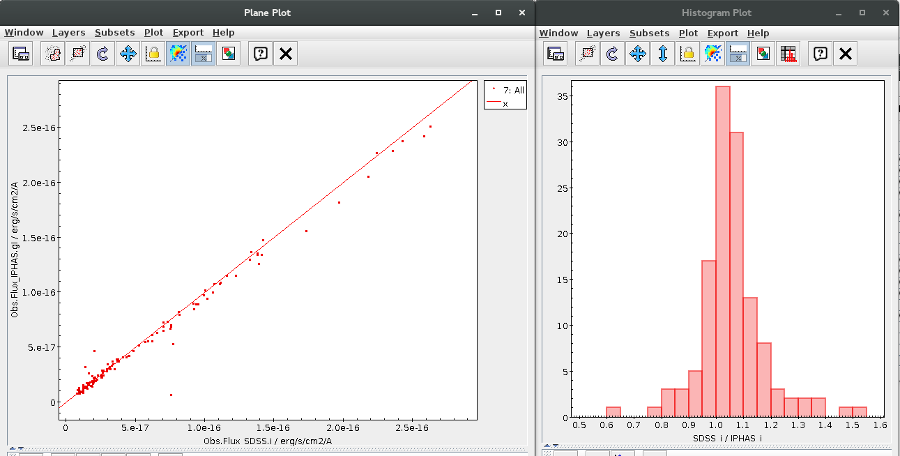
Flux comparison: SDSS DR9 / PanSTARRS DR1 (g,r,i,z bands)
$0<201 && contains(toString(q_mode),"+") && cl==6 && umag<22.0 && gmag<22.2 && rmag<22.2 && imag<21.3 && e_umag<0.2 && e_gmag<0.2 && e_rmag<0.2 && e_imag<0.2 && qualityflag<64 && gMeanApMagErr<0.2 && rMeanApMagErr<0.2 && iMeanApMagErr<0.2 && zMeanApMagErr<0.2 && gMeanApMag<23.3 && rMeanApMag<23.2 && iMeanApMag<23.1 && zMeanApMag<22.3
band
g
r
i
z
Median (SDSS/VPHAS+)
0.994
1.011
1.051
---
Q10 (SDSS/VPHAS+)
0.924
0.972
1.013
---
Q90 (SDSS/VPHAS+)
1.043
1.032
1.105
---
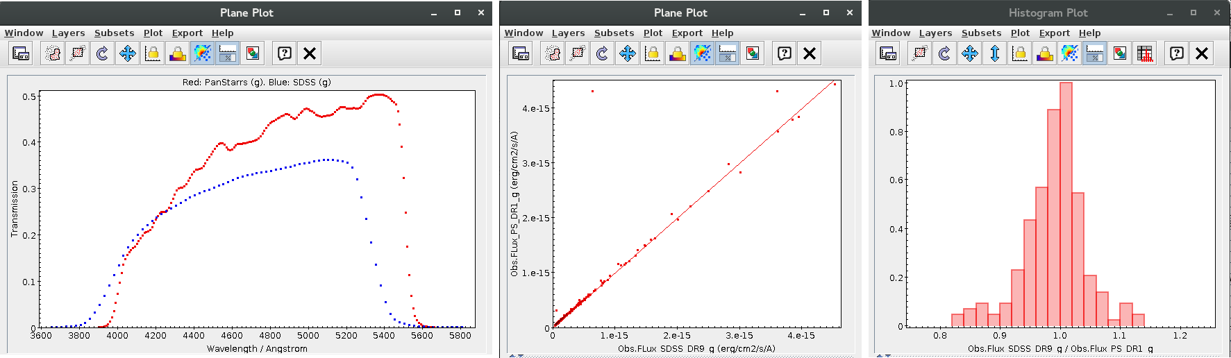
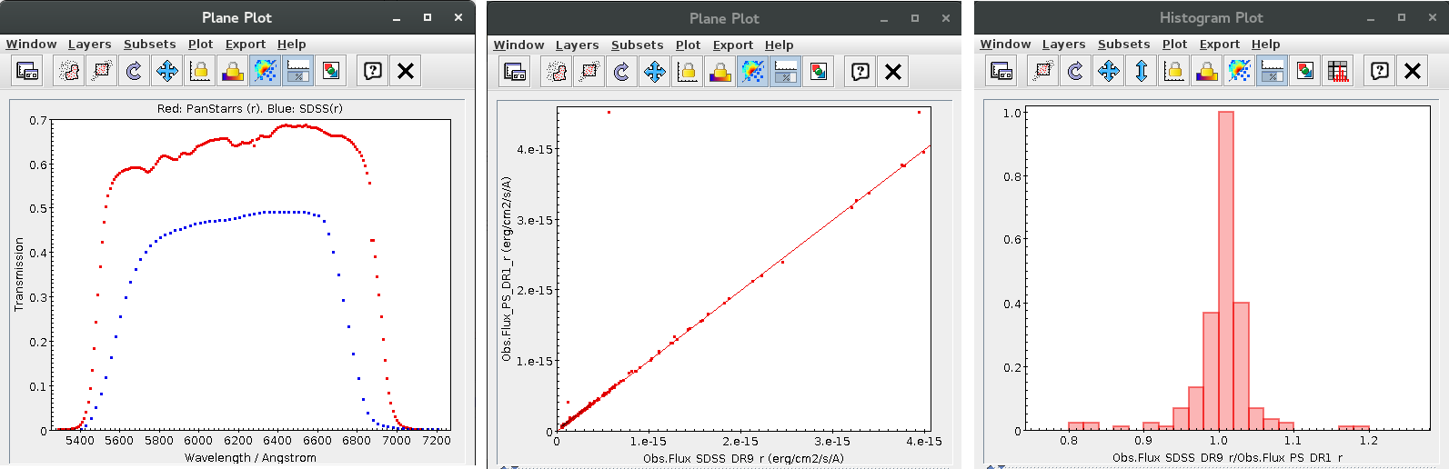
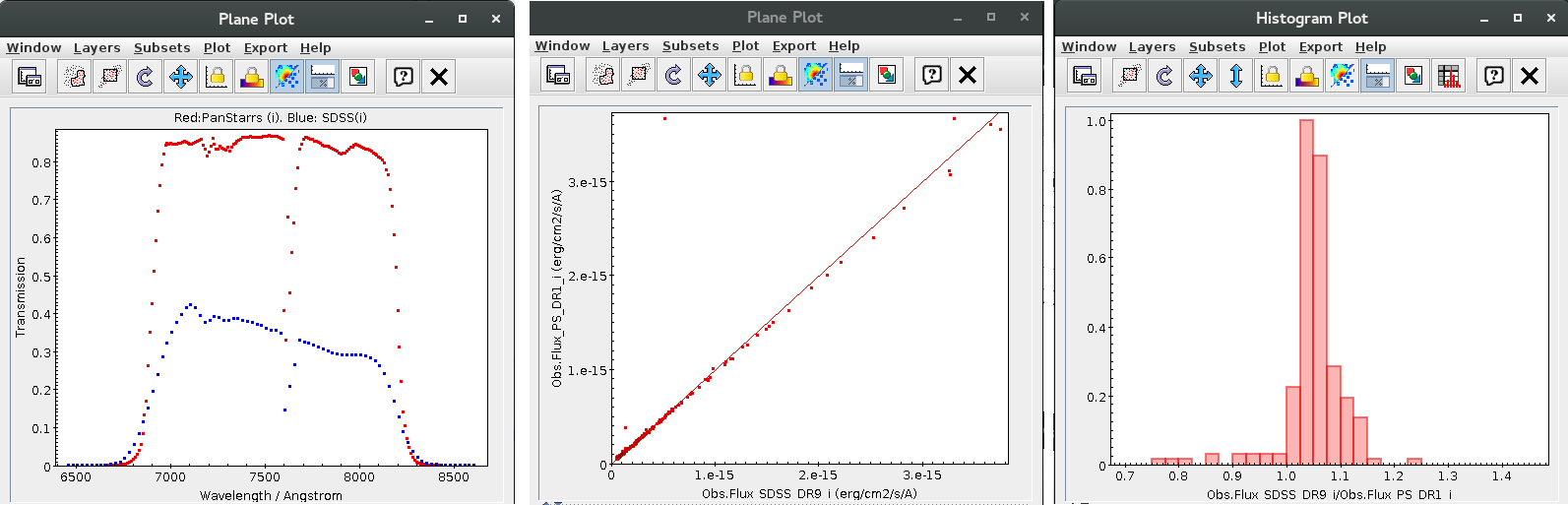
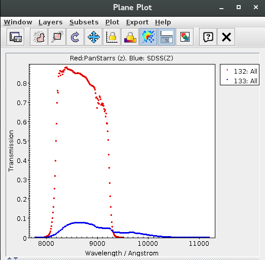
Flux comparison: SDSS DR9 / VPHAS DR2 (u,g,r,i bands)
$0<3000 && umag<22.0 && gmag<22.2 && rmag<22.2 && imag<21.3 && e_umag<0.2 && e_gmag<0.2 && e_rmag<0.2 && e_imag<0.2 && qmode && cl==6 && umag_x<22.0 && gmag_x<22.0 && rmag_x<22.0 && imag_x<22.0 && e_umag_x<0.2 && e_gmag_x<0.2 && e_rmag_x<0.2 && e_imag_x<0.2 && clean
band
u
g
r
i
Median (SDSS/VPHAS+)
0.851
1.023
1.048
1.030
Q10 (SDSS/VPHAS+)
0.701
0.973
1.008
0.977
Q90 (SDSS/VPHAS+)
0.953
1.063
1.085
1.075
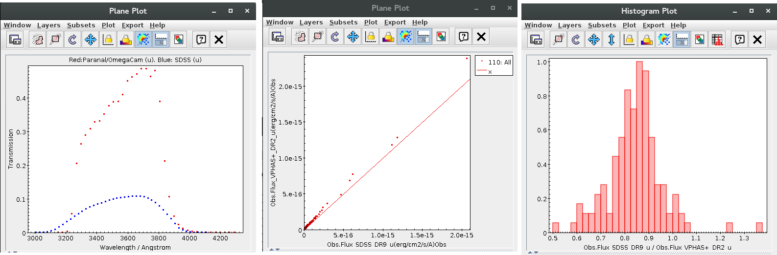
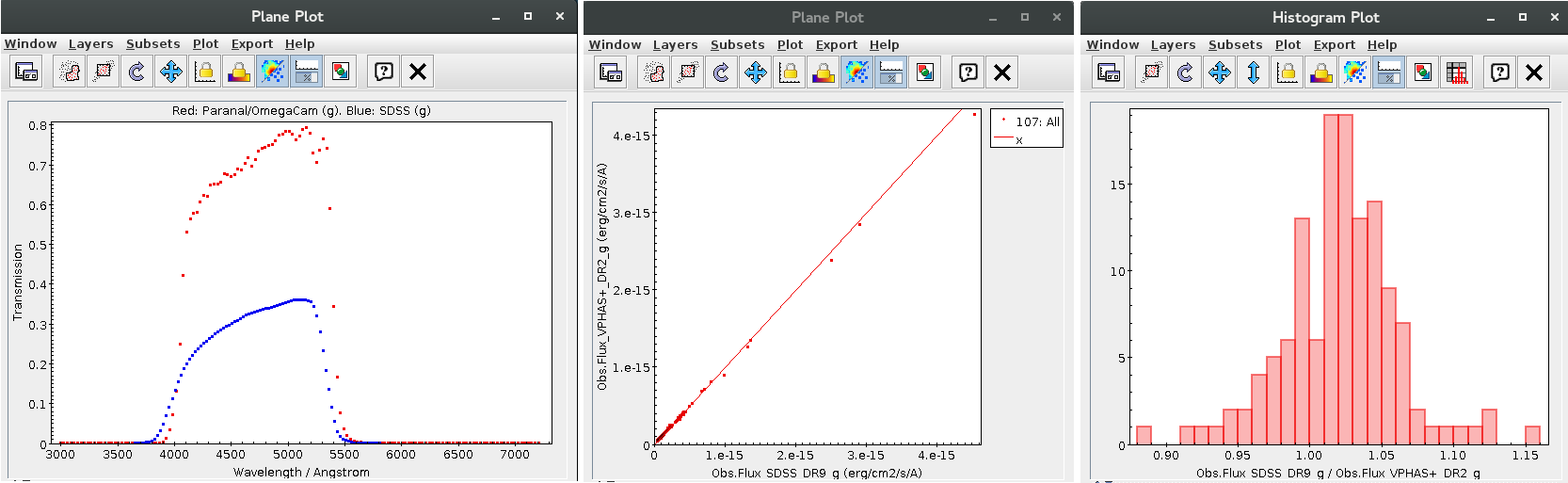

>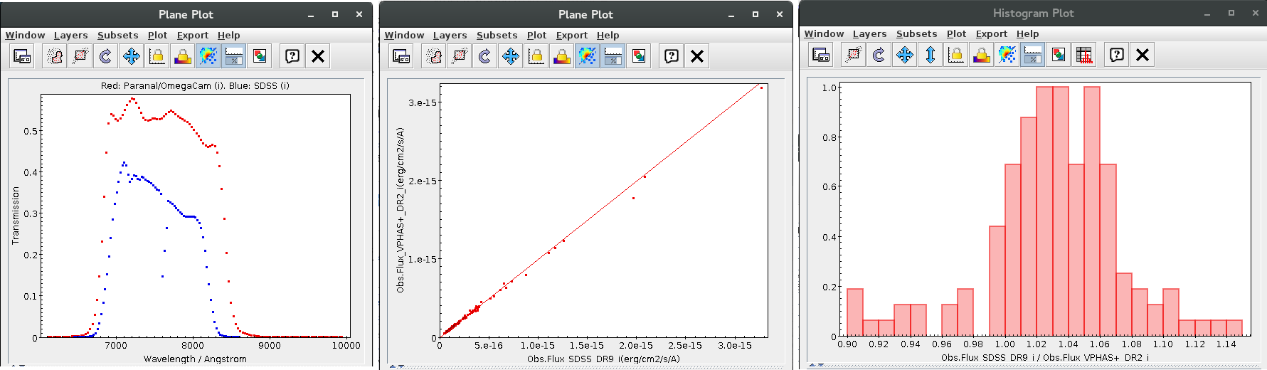
XMM testing with VOSA
Summary
We tested the XMM-OM Serendipitous Source Survey Catalogue 1 [XMM-
SUSS4.1, Page et al., 2012] in VOSA. To do that, we selected "good" sources from the catalogue with counterpart in GALEX DR2 AIS (All-sky Imaging
Survey) [Bianchi et al., 2011]. On one hand, we compared the observed fluxes in XMM filters with the theoretical fluxes predicted by the model, aiming
at proving their good fitting to the theoretical SED. On the other hand, we
compared the observed fluxes in XMM filters with fluxes in similar filters in
the ultraviolet and the optical wavelenght range.
Methodology
q.UVW2=="FFFFFFFFFFFF" && q.uVM2=="FFFFFFFFFFFF" && q.UVW1=="FFFFFFFFFFFF"
&& q.U=="FFFFFFFFFFFF" && q.B=="FFFFFFFFFFFF" && q.V=="FFFFFFFFFFFF"
&& xUVW2==0 && xUVM2==0 && xUVW1==0 && xU==0 && xB==0 && xV=0
&& e_UVW2mAB<=0.2 && e_UVM2mAB<=0.2 && e_UVW1mAB<=0.2 && e_UmAB<=0.2
&& e_BmAB<=0.2 && e_VmAB<=0.2
Flux comparison
UVW2
UVM2
UVW1
U
B
V
Median (F Obs /F Mod)
1.32
1.23
1.04
1.00
0.94
1.03
Q10 (F Obs /F Mod)
0.97
0.98
0.97
0.95
0.89
0.97
Q90 (F Obs /F Mod)
2.13
1.52
1.18
1.06
0.99
1.08
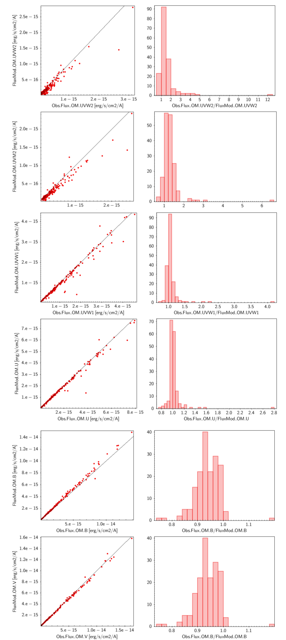
Figures 1 & 2: Comparison of observed and theoretical fluxes.
UVM2/NUV
BXMM/BAPASS
VXMM/VAPASS
Median (F Obs /F Mod)
1.15
0.97
1.03
Q10 (F Obs /F Mod)
0.91
0.90
0.95
Q90 (F Obs /F Mod)
1.38
1.06
1.10
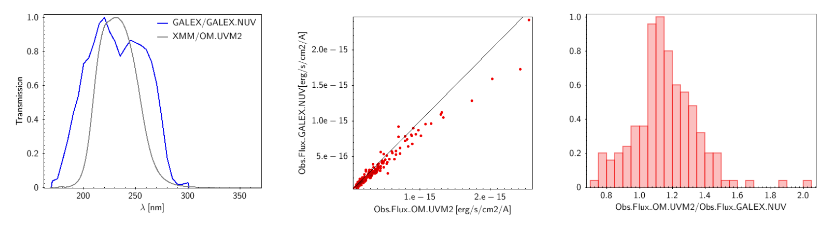
Figure 3: Comparison of filters and fluxes in the ultraviolet. 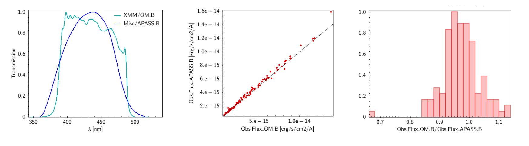
Figure 4: Comparison of filters and fluxes in the B band. 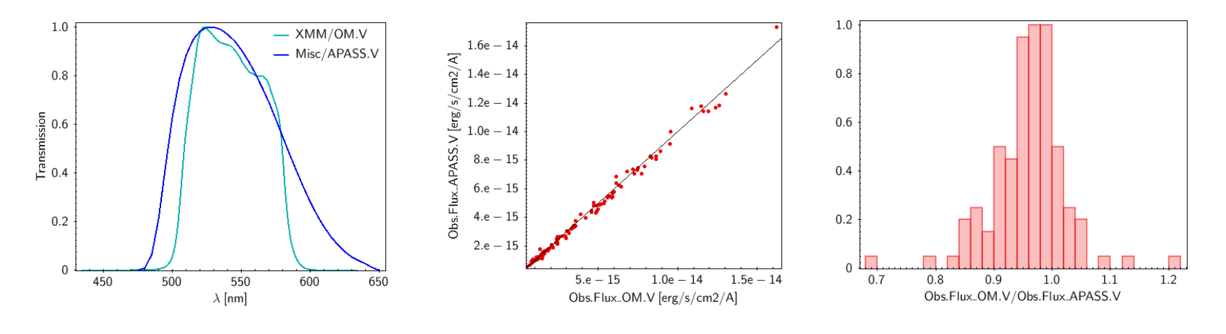
Figure 5: Comparison of filters and fluxes in the V band. Conclusions
In the ultraviolet the differences between observed and modeled fluxes are
larger than in the optical (see Table 1).
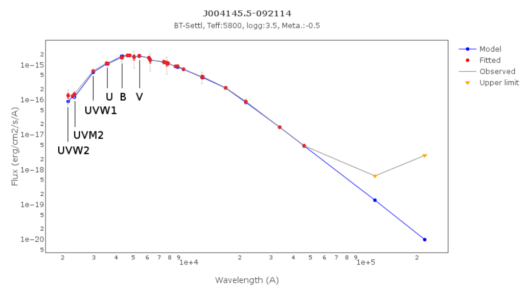
Figure 6: Example References
Assessment of the GALEX GR5/MIS fluxes.
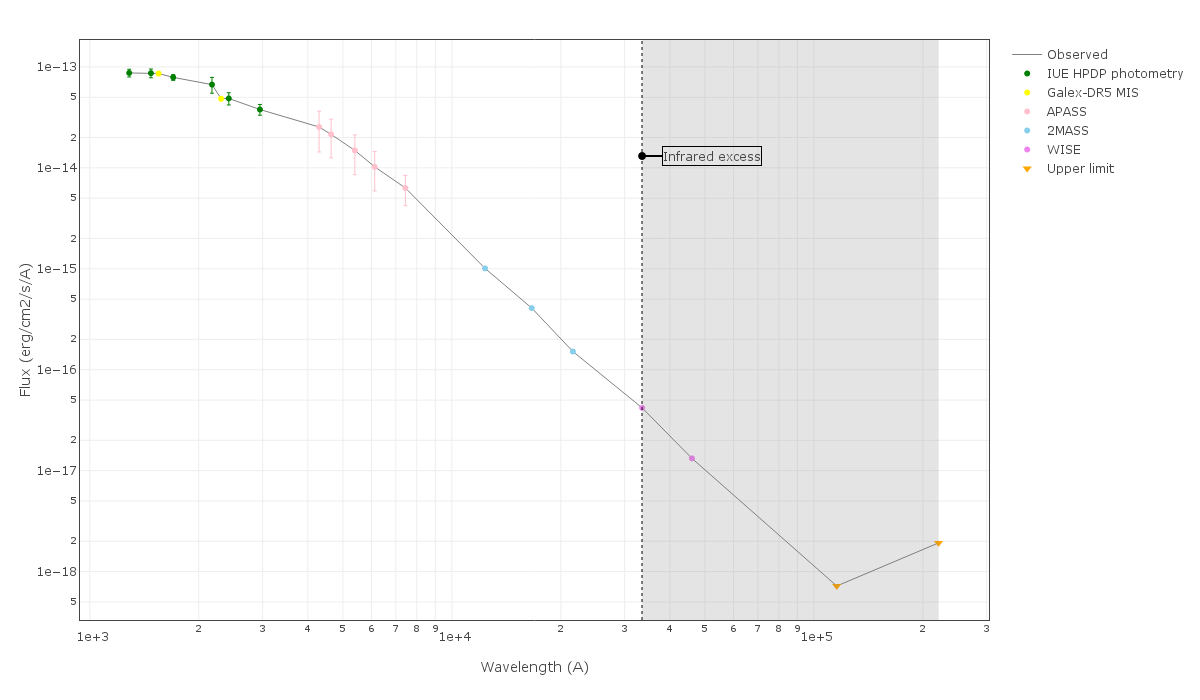
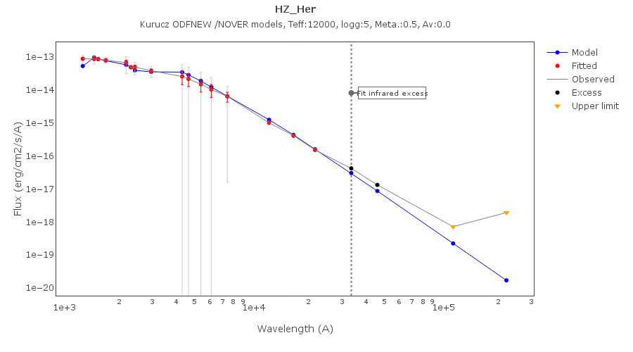
Assessment of the GALEX GR6+7 fluxes.
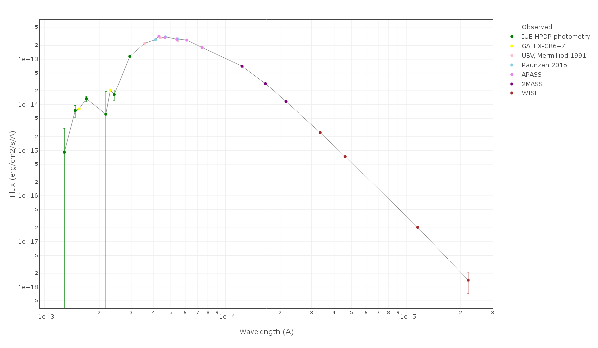
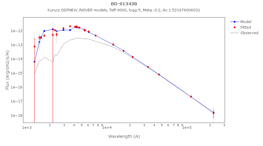
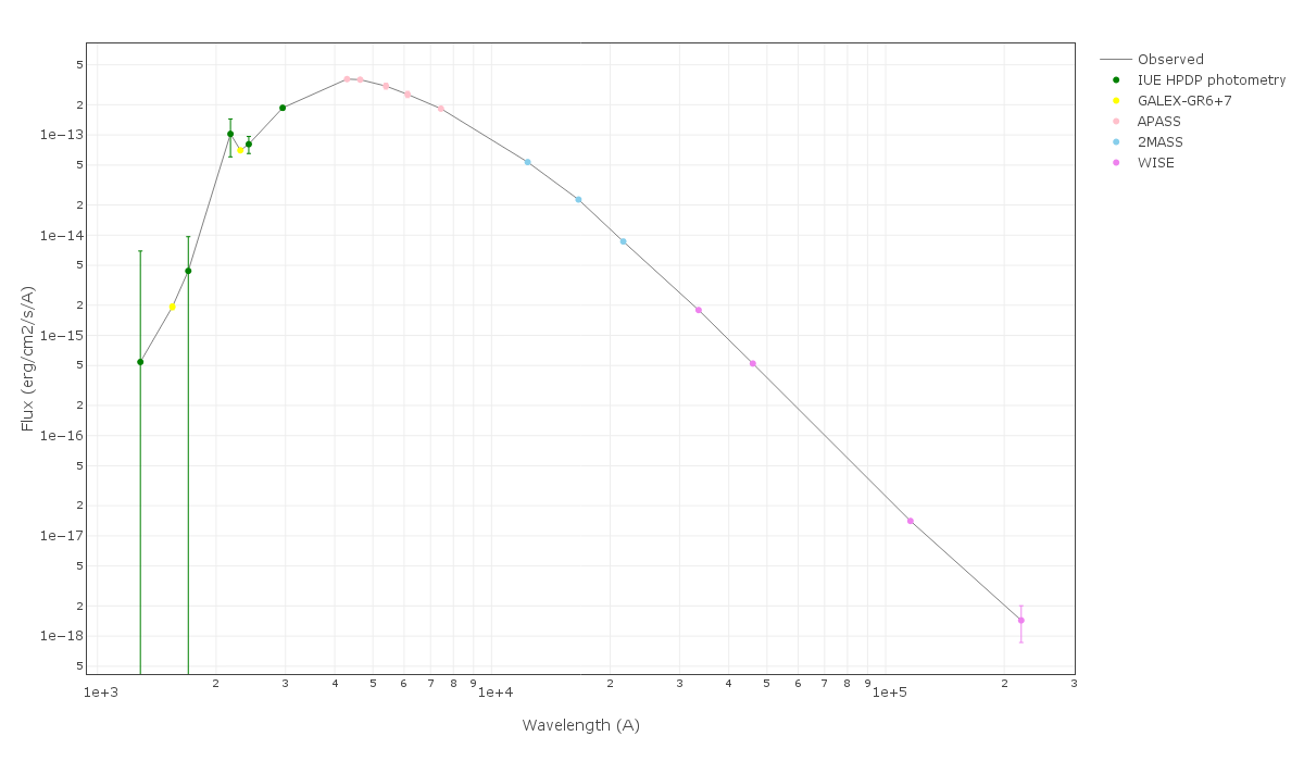
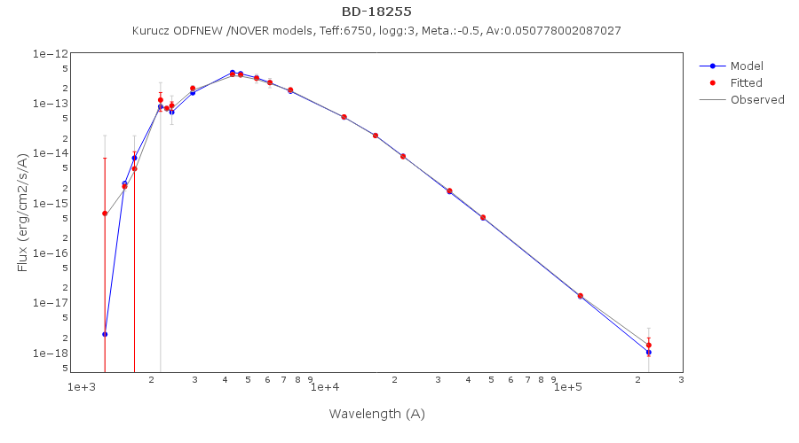
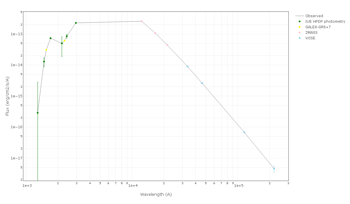
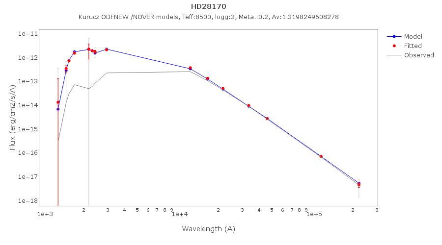
VOSA binary fit. Quality assurance testing. July 2023
Aim
FGK Spectral types
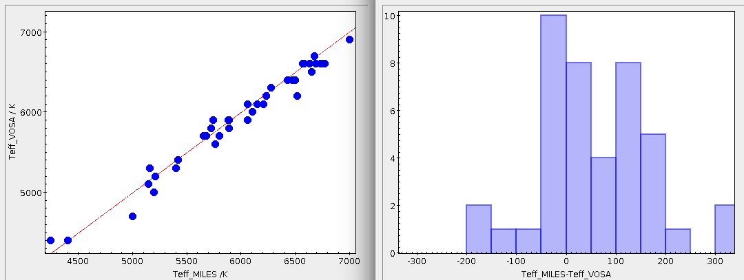
White dwarfs
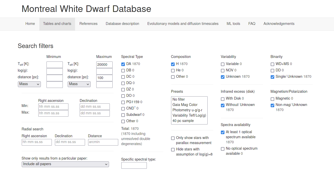

M stars
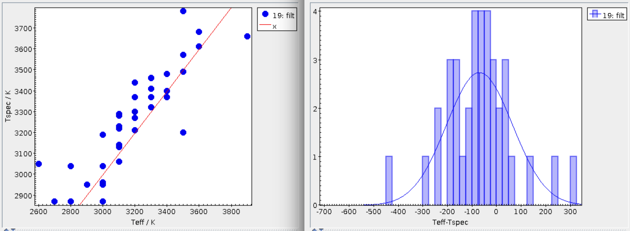
Binary fit use case #1
Hot white dwarf + FGK main sequence star (Parsons et al. 2016)
we see how 7 out of 8 objects show a clear excess in the blue, at GALEX and U_Johnson/u_SDSS bands, which indicates the presence of a second, hotter companion (the white dwarf in our case).
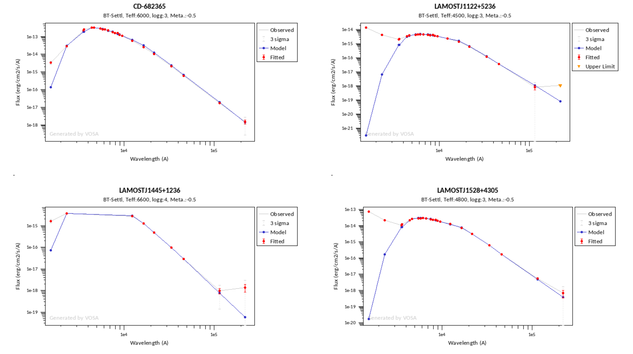
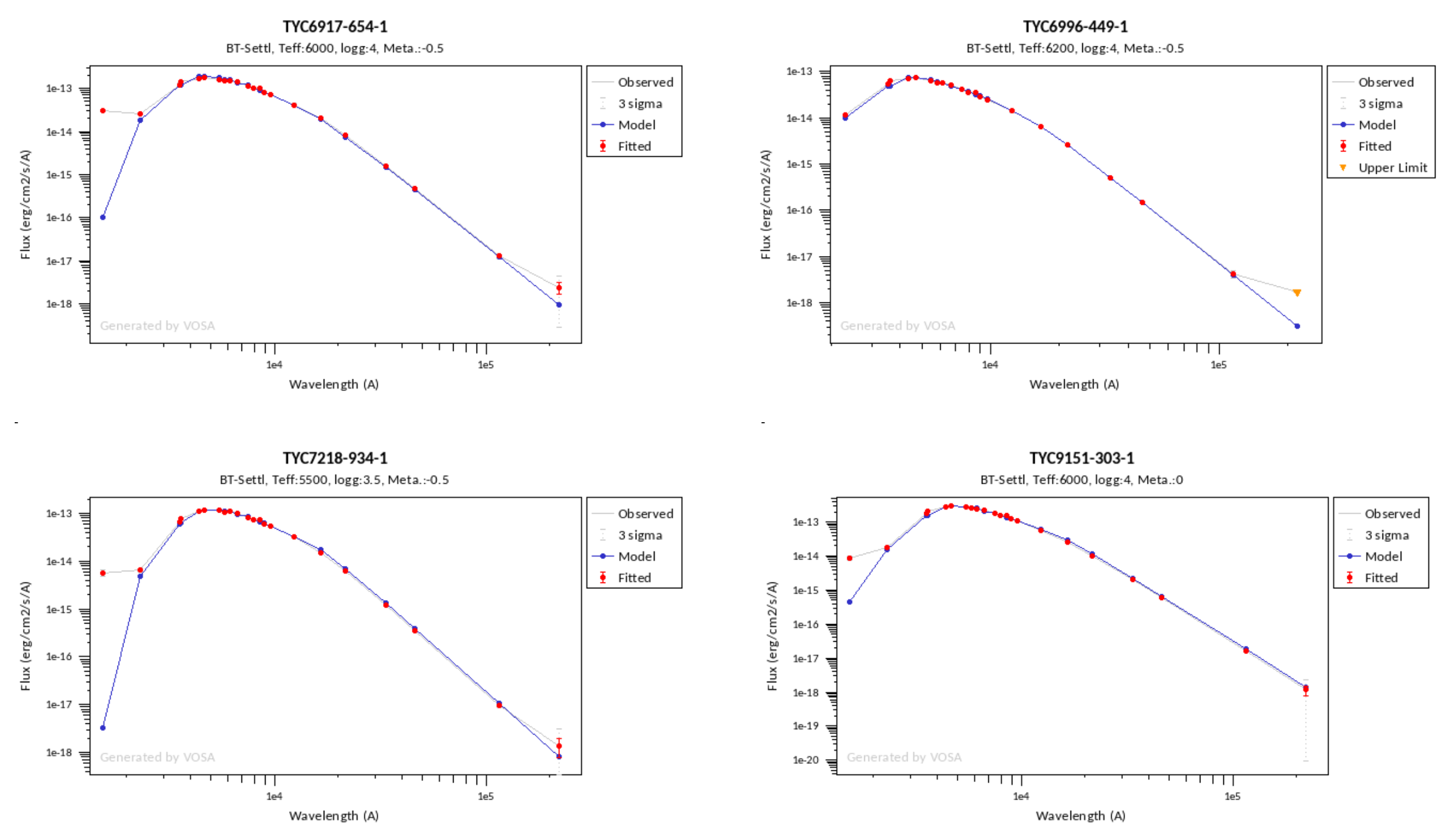
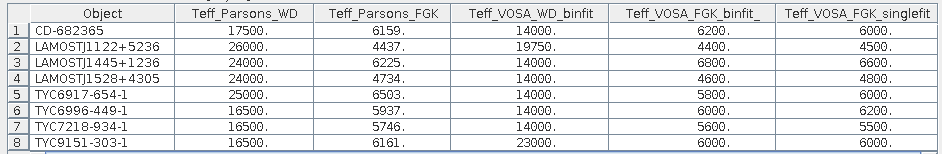
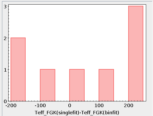
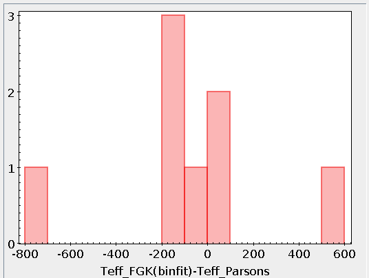
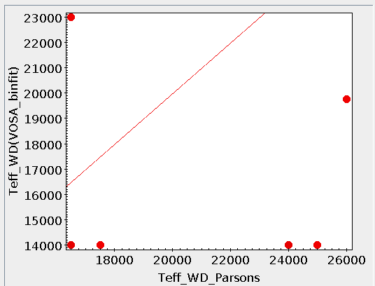
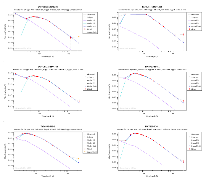
Binary fit use case #2
White dwarf + disk/brown dwarf
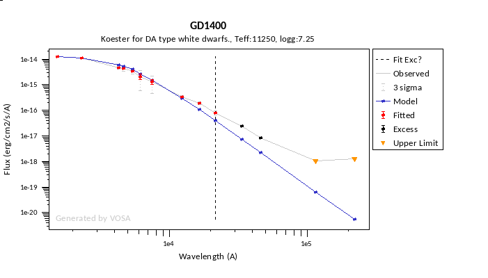
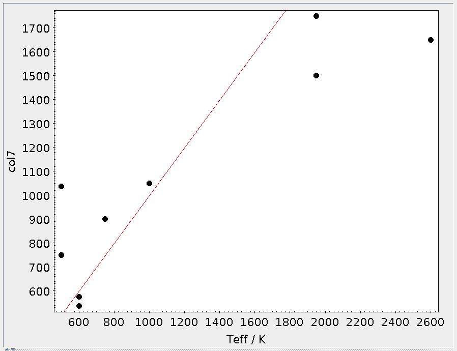
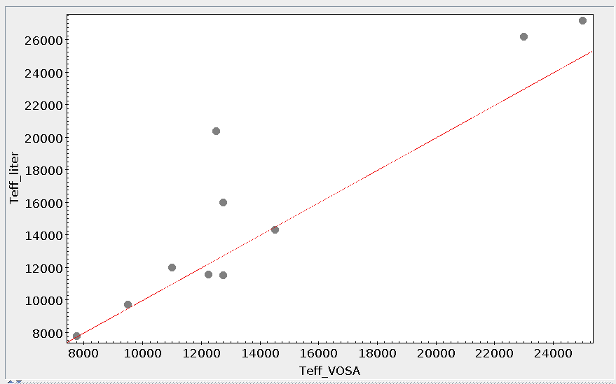
Binary fit use case #3
M dwarf + M dwarf
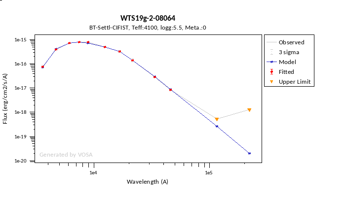
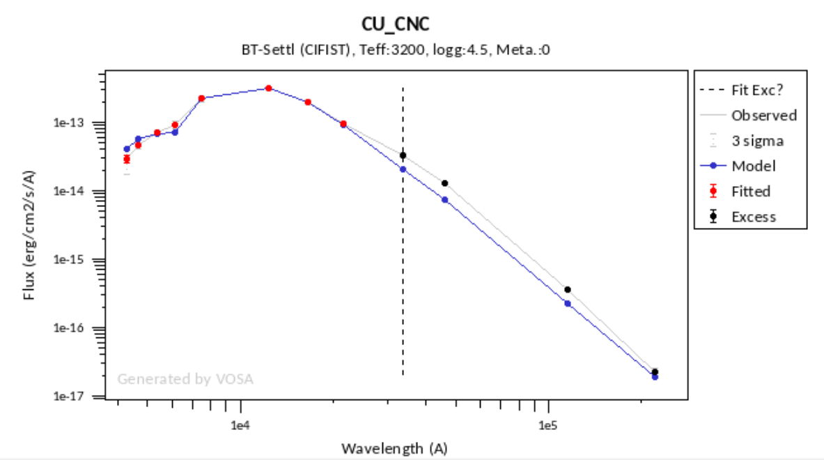
Credits
VOSA
This publication makes use of VOSA, developed under the Spanish Virtual Observatory (https://svo.cab.inta-csic.es) project funded by MCIN/AEI/10.13039/501100011033/ through grant PID2020-112949GB-I00.
Bayo, A., Rodrigo, C., Barrado y Navascués, D., Solano, E., Gutiérrez, R., Morales-Calderón, M., Allard, F. 2008, A&A 492,277B.
Theoretical Spectra.
Schryber, Miller & Tennyson 1995
Hauschildt et al 1999, ApJ 512, 377
Grevesse et al. 1993, A&A 271, 587
Baraffe et al 1998, A&A 337, 403B
Baraffe et al 1997, A&A 327, 1054
Allard et al 1997, ARA&A 35, 137
Partridge & Schwenke 1997
Grevesse et al. 1993, A&A 271, 587
Chabrier et al 2000, ApJ 542, 464C
Allard et al 2001, ApJ 556, 357A
Partridge & Schwenke 1997
Grevesse et al. 1993, A&A 271, 587
Baraffe et al 2003, A&A 402,701B
Allard et al 2001, ApJ 556, 357A
Castelli et al 1997, AA 318, 841
Castelli and Kurucz 2003, IAUS 210, A20
Castelli and Kurucz 2003, IAUS 210, A20
Barber et al 2006, MNRAS 368, 1087
Asplund et al. 2009, A&A 47, 481
Allard et al. 2013, MSAIS 24, 128
Allard et al 2012, RSPTA 370. 2765A
Allard et al 2011, ASPC 448, 91A
Allard et al 2007, A&A 474L, 21
Allard et al 2003, IAUS 211, 325
Barber et al 2006, MNRAS 368, 1087
Asplund et al. 2009, A&A 47, 481
Allard et al. 2013, MSAIS 24, 128
Allard et al 2012, RSPTA 370. 2765A
Allard et al 2011, ASPC 448, 91A
Allard et al 2007, A&A 474L, 21
Allard et al 2003, IAUS 211, 325
Caffau et al. 2011, SoPh 268, 255
Barber et al 2006, MNRAS 368, 1087
Allard et al. 2013, MSAIS 24, 128
Allard et al 2012, RSPTA 370. 2765A
Allard et al 2011, ASPC 448, 91A
Allard et al 2007, A&A 474L, 21
Allard et al 2003, IAUS 211, 325
Grevesse et al. 1993, A&A 271, 587
Barber et al 2006, MNRAS 368, 1087
Allard et al. 2013, MSAIS 24, 128
Allard et al 2012, RSPTA 370. 2765A
Allard et al 2011, ASPC 448, 91A
Allard et al 2007, A&A 474L, 21
Allard et al 2003, IAUS 211, 325
Caffau et al. 2011, SoPh 268, 255
Barber et al 2006, MNRAS 368, 1087
Allard et al 2012, RSPTA 370. 2765A
Allard et al 2011, ASPC 448, 91A
Caffau et al. 2011, SoPh 268, 255
Barber et al 2006, MNRAS 368, 1087
Allard et al 2012, RSPTA 370. 2765A
Allard et al 2011, ASPC 448, 91A
Barber et al 2006, MNRAS 368, 1087
Asplund et al. 2009, A&A 47, 481
Allard et al 2012, RSPTA 370. 2765A
Allard et al 2011, ASPC 448, 91A
Grevesse et al. 1993, A&A 271, 587
Barber et al 2006, MNRAS 368, 1087
Allard et al 2012, RSPTA 370. 2765A
Allard et al 2011, ASPC 448, 91A
Coelho 2014, MNRAS 440, 1027C
Koester, D. 2010; MSAI 81, 921
Trembley & Bergeron 2010, ApJ696, 1755
Levenhagen et al., 2017, ApJS 231, 1
Woitke P., Helling C., 2003, A&A, 399, 297
Witte et al. 2011, A&A, 529, A44
Witte et al. 2009, A&A, 506, 1367
Helling et al. 2008, ApJL, 675, L105
Helling et al. 2008, A&A, 485, 547
Helling C., Woitke P., 2006, A&A, 455, 325
Hauschildt & Baron 1999, JCoAM 109, 41
Baron et al. 2003, IAU 210, 19
Woitke P., Helling C., 2004, A&A, 414, 335
Morley et al. 2012, ApJ 756, 172
Morley et al. 2014, ApJ 789L, 14M
Morley et al. 2014, ApJ 787, 78M
Phillips et al 2020, eprint arXiv:2003.13717
Phillips et al 2020, eprint arXiv:2003.13717
Phillips et al 2020, eprint arXiv:2003.13717
Saumon et al. 2012, ApJ 750, 745
Rauch & Deetjen 2003, ASPC 288, 103R
Werner & Dreizler 1999, JCAM 109, 65
Werner at al. 2003, ASPC 288, 31W
Werner & Dreizler 1999, JCAM 109, 65
Rauch & Deetjen 2003, ASPC 288, 103R
Werner at al. 2003, ASPC 288, 31W
Werner & Dreizler 1999, JCAM 109, 65
Rauch & Deetjen 2003, ASPC 288, 103R
Werner at al. 2003, ASPC 288, 31W
Rauch & Deetjen 2003, ASPC 288, 103R
Werner at al. 2003, ASPC 288, 31W
Werner & Dreizler 1999, JCAM 109, 65
Rauch & Deetjen 2003, ASPC 288, 103R
Werner at al. 2003, ASPC 288, 31W
Werner & Dreizler 1999, JCAM 109, 65
Rauch & Deetjen 2003, ASPC 288, 103R
Werner at al. 2003, ASPC 288, 31W
Srinivasan et al. 2011, A&A, 532, A54
Sargent et al 2011, ApJ 728, 93
Husfeld et al 1989, A&A, 222, 150H
Pacheco et al. 2021, ApJS 256, 41P
Lanz, T., Hubeny, I. 2007, ApJS, 169, 83
Lanz, T., Hubeny, I. 2003, ApJS, 146, 417
Hubeny, I., Lanz, T. 1995, ApJ, 439, 875HTemplate fit
Bayo et al 2011, A&A 536, 63B
Rajpurohit et al. 2012, A&A 545A, 85R
Rajpurohit et al 2014, eprint asXiv: 1401.2901R
Knapp et al. 2004, AJ, 127, 3553
Golimowski et al. 2004, AJ, 127, 3516
Chiu et al. 2006, AJ, 131, 2722
Kirkpatrick et al. 1999, ApJ, 519, 802
Kirkpatrick et al 1991, ApJS, 77, 417
McLean et al. 2003, ApJ 596, 561M
McLean et al. 2007, ApJ 658, 1217
Kesseli et al 2017Theoretical Isochrones and Evolutionary Tracks
Baraffe et al. 2015, arXiv:1503.04107
Baraffe et al 2002, A&A 385, 563
Baraffe et al 1998, A&A 337, 403B
Baraffe et al 2003, A&A 402,701B
Chabrier et al 2000, ApJ 542, 464C
Baraffe et al 2002, A&A 385, 563
Siess et al 2000, A&A, 358, 593S
Bressan et al. 2016, MNRAS 427,127
Ekström & al. (2012) A&A 537, A146
Georgy & al. (2012) A&A 542, A29
Georgy et al. (2013) A&A 558, A103
Groh et al. (2019) A&A 627, A24
Haemmerlé et al. (2019) A&A 624, A137
Somers et al, 2020, ApJ 891, 29
Somers et al, 2020, ApJ 891, 29
Somers et al, 2020, ApJ 891, 29
Somers et al, 2020, ApJ 891, 29
Somers et al, 2020, ApJ 891, 29
Somers et al, 2020, ApJ 891, 29
Phillips et al 2020, eprint arXiv:2003.13717
Phillips et al 2020, eprint arXiv:2003.13717
Phillips et al 2020, eprint arXiv:2003.13717VO Photometry
Skrutskie et al, 2006, AJ, 131, 1163S
Ochsenbein et al 2000, A&AS 143, 221
This publication makes use of data products from the Two Micron All Sky Survey, which is a joint project of the University of Massachusetts and the Infrared Processing and Analysis Center/California Institute of Technology, funded by the National Aeronautics and Space Administration and the National Science Foundation.
Ishihara et al, 2010, A&A, 514, A1
Murakami et al, 2007, PASJ 59, S369
Ochsenbein et al 2000, A&AS 143, 221
Onaka et al, 2007, PASJ, 59, S401
Kawada et al, 2007, PASJ, 59, S389
Murakami et al, 2007, PASJ 59, S369
Ochsenbein et al 2000, A&AS 143, 221
This publication makes use of data products from the Wide-field Infrared Survey Explorer, which is a joint project of the University of California, Los Angeles, and the Jet Propulsion Laboratory/California Institute of Technology, funded by the National Aeronautics and Space Administration.
Ochsenbein et al 2000, A&AS 143, 221
Wright et al 2010, AJ 140, 1868W
Ochsenbein et al 2000, A&AS 143, 221
Fouque et al. 2000, A&AS 141, 313F
Epchtein et al. 1999, A&A 349, 236E
Benjamin et al. 2003, PASP 115, 953B
Churchwell et al. 2009, PASP 121, 213C
Ochsenbein et al 2000, A&AS 143, 221
Helou, G. & Walker, D.W.; Infrared astronomical satellite (IRAS) catalogs and atlases. Volume 7, p.1-265
Beichman et al. 1988, IRAS vol I
Ochsenbein et al 2000, A&AS 143, 221
Beichman et al. 1988, IRAS vol I
Helou, G. & Walker, D.W.; Infrared astronomical satellite (IRAS) catalogs and atlases. Volume 7, p.1-265
Ochsenbein et al 2000, A&AS 143, 221
Evans et al, 2003, PASP, 115, 965E
Evans et al. 2009, ApJS 181, 321E
Carpenter et al. 2008, ApJS 2008, 179, 423C
McCabe et al 2009, AAS 21343905M
cat:MSX catalogue
Ochsenbein et al 2000, A&AS 143, 221
Mainzer et al. 2014, ApJ, 792, 30
This publication makes use of data products from the Near-Earth Object Wide-field Infrared Survey Explorer (NEOWISE), which is a joint project of the Jet Propulsion Laboratory/California Institute of Technology and the University of Arizona. NEOWISE is funded by the National Aeronautics and Space Administration.
Hodgkin et ak, 2009, MNRAS, 394, 675
Hewett et al 2006, MNRAS, 367, 454
Hambly et al 2008, MNRAS 384, 637
Casali et al, 2007, A&A, 467, 777
Lawrence et al, 2007, MNRAS, 379, 1599
Hodgkin et ak, 2009, MNRAS, 394, 675
Hewett et al 2006, MNRAS, 367, 454
Hambly et al 2008, MNRAS 384, 637
Casali et al, 2007, A&A, 467, 777
Lawrence et al, 2007, MNRAS, 379, 1599
Hodgkin et ak, 2009, MNRAS, 394, 675
Hewett et al 2006, MNRAS, 367, 454
Hambly et al 2008, MNRAS 384, 637
Casali et al, 2007, A&A, 467, 777
Lawrence et al, 2007, MNRAS, 379, 1599
Hodgkin et ak, 2009, MNRAS, 394, 675
Hewett et al 2006, MNRAS, 367, 454
Hambly et al 2008, MNRAS 384, 637
Casali et al, 2007, A&A, 467, 777
Lawrence et al, 2007, MNRAS, 379, 1599
Hodgkin et ak, 2009, MNRAS, 394, 675
Hewett et al 2006, MNRAS, 367, 454
Hambly et al 2008, MNRAS 384, 637
Casali et al, 2007, A&A, 467, 777
Lawrence et al, 2007, MNRAS, 379, 1599
Cross et al. 2009, MNRAS 399, 1730C
Cross et al. 2012, A&A 548, 119C
Hambly et al 2008, MNRAS 384, 637
Irwin et al. 2004, SPIE 5493, 411
Cross et al. 2009, MNRAS 399, 1730C
Cross et al. 2012, A&A 548, 119C
Hambly et al 2008, MNRAS 384, 637
Irwin et al. 2004, SPIE 5493, 411
Cross et al. 2009, MNRAS 399, 1730C
Cross et al. 2012, A&A 548, 119C
Hambly et al 2008, MNRAS 384, 637
Irwin et al. 2004, SPIE 5493, 411
Cross et al. 2009, MNRAS 399, 1730C
Cross et al. 2012, A&A 548, 119C
Hambly et al 2008, MNRAS 384, 637
Irwin et al. 2004, SPIE 5493, 411
Cross et al. 2009, MNRAS 399, 1730C
Cross et al. 2012, A&A 548, 119C
Hambly et al 2008, MNRAS 384, 637
Irwin et al. 2004, SPIE 5493, 411
Cristóbal-Hornillos et al. 2009, ApJ 696, 1554
Moles et al, AJ, 2008, 136, 1325
Molino et al. 2013, MNRAS 441,2891
Villegas et al. 2010, AJ 139, 1242
Evans et al. 2002, A&A 395, 347E
Ochsenbein et al 2000, A&AS 143, 221
Ochsenbein et al 2000, A&AS 143, 221
Ochsenbein et al 2000, A&AS 143, 221
Ochsenbein et al 2000, A&AS 143, 221
This project used public archival data from the Dark Energy Survey (DES). Funding for the DES Projects has been provided by the U.S. Department of Energy, the U.S. National Science Foundation, the Ministry of Science and Education of Spain, the Science and Technology Facilities Council of the United Kingdom, the Higher Education Funding Council for England, the National Center for Supercomputing Applications at the University of Illinois at UrbanaChampaign, the Kavli Institute of Cosmological Physics at the University of Chicago, the Center for Cosmology and Astro-Particle Physics at the Ohio State University, the Mitchell Institute for Fundamental Physics and Astronomy at Texas A&M University, Financiadora de Estudos e Projetos, Fundação Carlos Chagas Filho de Amparo à Pesquisa do Estado do Rio de Janeiro, Conselho Nacional de Desenvolvimento Científico e Tecnológico and the Ministério da Ciência, Tecnologia e Inovação, the Deutsche Forschungsgemeinschaft and the Collaborating Institutions in the Dark Energy Survey.
The Collaborating Institutions are Argonne National Laboratory, the University of California at Santa Cruz, the University of Cambridge, Centro de Investigaciones Enérgeticas, Medioambientales y TecnológicasMadrid, the University of Chicago, University College London, the DES-Brazil Consortium, the University of Edinburgh, the Eidgenössische Technische Hochschule (ETH) Zürich, Fermi National Accelerator Laboratory, the University of Illinois at Urbana-Champaign, the Institut de Ciències de l'Espai (IEEC/CSIC), the Institut de Física d'Altes Energies, Lawrence Berkeley National Laboratory, the Ludwig-Maximilians Universität München and the associated Excellence Cluster Universe, the University of Michigan, the National Optical Astronomy Observatory, the University of Nottingham, The Ohio State University, the OzDES Membership Consortium, the University of Pennsylvania, the University of Portsmouth, SLAC National Accelerator Laboratory, Stanford University, the University of Sussex, and Texas A&M University.
Based in part on observations at Cerro Tololo Inter-American Observatory, National Optical Astronomy Observatory, which is operated by the Association of Universities for Research in Astronomy (AURA) under a cooperative agreement with the National Science Foundation.
Abbott et al. 2018, ApJS 239 18A
Gaia DR3 Credit and citation instructions
Gaia DR3 Documentation
Ochsenbein et al 2000, A&AS 143, 221
Gaia, Montegriffo et al. 2022
Gaia Collaboration et al. 2016, A&A 595, 1G
This work has made use of data from the European Space Agency (ESA) mission Gaia (https://www.cosmos.esa.int/gaia), processed by the Gaia Data Processing and Analysis Consortium (DPAC, https://www.cosmos.esa.int/web/gaia/dpac/consortium). Funding for the DPAC has been provided by national institutions, in particular the institutions participating in the Gaia Multilateral Agreement.
Gaia DR3 Documentation
Gaia DR3 Credit and citation instructions
Ochsenbein et al 2000, A&AS 143, 221
Gaia Collaboration et al. 2016, A&A 595, 1G
This work has made use of data from the European Space Agency (ESA) mission Gaia (https://www.cosmos.esa.int/gaia), processed by the Gaia Data Processing and Analysis Consortium (DPAC, https://www.cosmos.esa.int/web/gaia/dpac/consortium). Funding for the DPAC has been provided by national institutions, in particular the institutions participating in the Gaia Multilateral Agreement.
Gaia DR3 Documentation
Gaia DR3 Credit and citation instructions
Gaia, Montegriffo et al. 2022
Gaia Collaboration et al. 2016, A&A 595, 1G
This work has made use of data from the European Space Agency (ESA) mission Gaia (https://www.cosmos.esa.int/gaia), processed by the Gaia Data Processing and Analysis Consortium (DPAC, https://www.cosmos.esa.int/web/gaia/dpac/consortium). Funding for the DPAC has been provided by national institutions, in particular the institutions participating in the Gaia Multilateral Agreement.
Cortés-Contreras et al, 2020, MNRAS 491, 129C
Barentsen et al, 2014, MNRAS 444, 3230B
González-Solares et al, 2008, MNRAS, 388, 89G
Ochsenbein et al 2000, A&AS 143, 221
Ochsenbein et al 2000, A&AS 143, 221
Paunzen, 2015, A&A 580A, 23P
Waters et al 2016, arXiv: 1612.05245
Magnier et al 2016, arXiv:1612.05242
Magnier et al 2016, arXiv:1612.05240
Magnier et al 2016, arXiv: 1612.05244
Flewelling et al 2016, arXiv: 1612.05243
Chambers et al 2016, arXiv: 1612.05560
The Pan-STARRS1 Surveys (PS1) and the PS1 public science archive have been made possible through contributions by the Institute for Astronomy, the University of Hawaii, the Pan-STARRS Project Office, the Max-Planck Society and its participating institutes, the Max Planck Institute for Astronomy, Heidelberg and the Max Planck Institute for Extraterrestrial Physics, Garching, The Johns Hopkins University, Durham University, the University of Edinburgh, the Queen's University Belfast, the Harvard-Smithsonian Center for Astrophysics, the Las Cumbres Observatory Global Telescope Network Incorporated, the National Central University of Taiwan, the Space Telescope Science Institute, the National Aeronautics and Space Administration under Grant No. NNX08AR22G issued through the Planetary Science Division of the NASA Science Mission Directorate, the National Science Foundation Grant No. AST-1238877, the University of Maryland, Eotvos Lorand University (ELTE), the Los Alamos National Laboratory, and the Gordon and Betty Moore Foundation.
Ochsenbein et al 2000, A&AS 143, 221
Alam et al., 2015, ApJS, 219, 12A
Funding for the SDSS and SDSS-II has been provided by the Alfred P. Sloan Foundation, the Participating Institutions, the National Science Foundation, the U.S. Department of Energy, the National Aeronautics and Space Administration, the Japanese Monbukagakusho, the Max Planck Society, and the Higher Education Funding Council for England. The SDSS Web Site is http://www.sdss.org/.
The SDSS is managed by the Astrophysical Research Consortium for the Participating Institutions. The Participating Institutions are the American Museum of Natural History, Astrophysical Institute Potsdam, University of Basel, University of Cambridge, Case Western Reserve University, University of Chicago, Drexel University, Fermilab, the Institute for Advanced Study, the Japan Participation Group, Johns Hopkins University, the Joint Institute for Nuclear Astrophysics, the Kavli Institute for Particle Astrophysics and Cosmology, the Korean Scientist Group, the Chinese Academy of Sciences (LAMOST), Los Alamos National Laboratory, the Max-Planck-Institute for Astronomy (MPIA), the Max-Planck-Institute for Astrophysics (MPA), New Mexico State University, Ohio State University, University of Pittsburgh, University of Portsmouth, Princeton University, the United States Naval Observatory, and the University of Washington.
Hauck, B.; Mermilliod, M., 1998A&AS, 129, 431
Ochsenbein et al 2000, A&AS 143, 221
Hog et al 2000 A&A 355, 27
Ochsenbein et al 2000, A&AS 143, 221
Ochsenbein et al 2000, A&AS 143, 221
Drew et al. 2014, MNRAS 440,2036
Ochsenbein et al 2000, A&AS 143, 221
Masci et al. 2019, PASP 131, 995
Based on observations obtained with the Samuel Oschin Telescope 48-inch and the 60-inch Telescope at the Palomar Observatory as part of the Zwicky Transient Facility project. ZTF is supported by the National Science Foundation under Grants No. AST-1440341 and AST-2034437 and a collaboration including current partners Caltech, IPAC, the Weizmann Institute for Science, the Oskar Klein Center at Stockholm University, the University of Maryland, Deutsches Elektronen-Synchrotron and Humboldt University, the TANGO Consortium of Taiwan, the University of Wisconsin at Milwaukee, Trinity College Dublin, Lawrence Livermore National Laboratories, IN2P3, University of Warwick, Ruhr University Bochum, Northwestern University and former partners the University of Washington, Los Alamos National Laboratories, and Lawrence Berkeley National Laboratories. Operations are conducted by COO, IPAC, and UW.
Ochsenbein et al 2000, A&AS 143, 221
Bianchi et al. 2011, AP&SS 335, 161B
Ochsenbein et al 2000, A&AS 143, 221
Bianchi et al. 2017, ApJS 230 24BObject coordinates
This research has made use of the SIMBAD database,
operated at CDS, Strasbourg, France
Wenger et al. 2000, A&AS 143, 9WObject distance VO services
Gaia Collaboration et al. 2018, A&A 616, A1
Gaia Collaboration et al. 2016, A&A 595, 1G
Evans et al. 2018, A&A 616 A4
This work has made use of data from the European Space Agency (ESA) mission Gaia (https://www.cosmos.esa.int/gaia), processed by the Gaia Data Processing and Analysis Consortium (DPAC, https://www.cosmos.esa.int/web/gaia/dpac/consortium). Funding for the DPAC has been provided by national institutions, in particular the institutions participating in the Gaia Multilateral Agreement.
Gaia DR3 Documentation
Gaia DR3 Credit and citation instructions
Ochsenbein et al 2000, A&AS 143, 221
Gaia Collaboration et al. 2016, A&A 595, 1G
This work has made use of data from the European Space Agency (ESA) mission Gaia (https://www.cosmos.esa.int/gaia), processed by the Gaia Data Processing and Analysis Consortium (DPAC, https://www.cosmos.esa.int/web/gaia/dpac/consortium). Funding for the DPAC has been provided by national institutions, in particular the institutions participating in the Gaia Multilateral Agreement.Dereddening
Fitzpatrick, E.; 1999, PASP, 111, 63
Indebetouw et al, 2005, ApJ 619, 931Extinction properties VO services
Gaia DR3 Documentation
Gaia DR3 Credit and citation instructions
Ochsenbein et al 2000, A&AS 143, 221
Gaia Collaboration et al. 2016, A&A 595, 1G
This work has made use of data from the European Space Agency (ESA) mission Gaia (https://www.cosmos.esa.int/gaia), processed by the Gaia Data Processing and Analysis Consortium (DPAC, https://www.cosmos.esa.int/web/gaia/dpac/consortium). Funding for the DPAC has been provided by national institutions, in particular the institutions participating in the Gaia Multilateral Agreement.
Denoyelle J. 1977, A&AS 27, 343
Ochsenbein et al 2000, A&AS 143, 221
Ochsenbein et al 2000, A&AS 143, 221
Glushkova E.V. et al, Astronomy Letters,36, 75 (2010)
Ochsenbein et al 2000, A&AS 143, 221
Guarinos J., Ph.D. Thesis, 1992
Guarinos 1992, ESO proceedings
Ochsenbein et al 2000, A&AS 143, 221
Gunn, J. E.; Stryker, L. L., 1983, ApJS, 52, 121
Ochsenbein et al 2000, A&AS 143, 221
Jones et al 2000, MNRAS, 399, 683J
Ochsenbein et al 2000, A&AS 143, 221
Kodaira et al 1992, National Astron. Obs. of Japan
Ochsenbein et al 2000, A&AS 143, 221
Larson K.A., Whittet D.C.B. 2005, ApJ, 623, 897
Ochsenbein et al 2000, A&AS 143, 221
Layden 1995. AJ. 110, 2288L
Ochsenbein et al 2000, A&AS 143, 221
Le Borgne et al 2003, Astron. Astrophys. 402, 433
Ochsenbein et al 2000, A&AS 143, 221
Ochsenbein et al 2000, A&AS 143, 221
Savage et al 1985, ApJS 99, 397S
Morales et al 2006, Lecture Notes and Essays in Astrophysics, vol. 2, p. 189-198.
Morales et al 2006, Lecture Notes and Essays in Astrophysics, vol. 2, p. 189-198.
Ochsenbein et al 2000, A&AS 143, 221
Rowan-Robinson 2008, MNRAS., 386, 697R
Kainulainen et al 2009, A&A 26, 508Helpdesk
About
VOSA
(VO Sed Analyzer)
Appendix A: IR excess detection examples
1.- A simple case
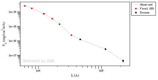
np FilterID Wavelength Flux ΔFlux log(nu) log(nuFnu) e_log(nuFnu) weight exc a b σa σb nsig b+σb<2.56 nsig>3
•
0 2MASS/2MASS.Ks 21590 1.3987756851941E-15 2.4478080312896E-17 14.1426 -10.52 0.0076 17313 --- --- --- --- --- --- --- --- •
1 WISE/WISE.W1 33526 2.4473412676635E-16 7.3027728843144E-18 13.9514 -11.0859 0.0129592 5954.49 --- -52.3955 2.96095 1.10782 0.078603 -5.91349 --- --- •
2 WISE/WISE.W2 46028 1.2557903316284E-16 2.313251278027E-18 13.8138 -11.2381 0.008 15625 1 -41.8432 2.21355 0.46764 0.0334457 15.4485 yes yes •
3 WISE/WISE.W3 115608 2.6104843027125E-17 5.770427751284E-19 13.4138 -11.5203 0.0096 10850.7 1 -29.4675 1.3353 0.231943 0.0167091 90.1323 yes yes •
4 WISE/WISE.W4 220883 4.0506648798552E-18 5.5962003414414E-19 13.1327 -12.0483 0.06 277.778 1 -39.3027 2.03245 0.691006 0.0490669 17.6176 yes yes Details, point by point
Points used for regression at WISE/WISE.W1: FilterID Wavelength Flux ΔFlux log(nu) log(nuFnu) e_log(nuFnu) weight
2MASS/2MASS.Ks
21590
1.3987756851941E-15
2.4478080312896E-17
14.1426
-10.52
0.0076
17313
WISE/WISE.W1
33526
2.4473412676635E-16
7.3027728843144E-18
13.9514
-11.0859
0.0129592
5954.49
b + σ(b) = 3.03956 > 2.56 ⇒ NO excess
yL= -11.0093
(yobs-yL)/σ(y) = -5.91349 ⇒ NO excess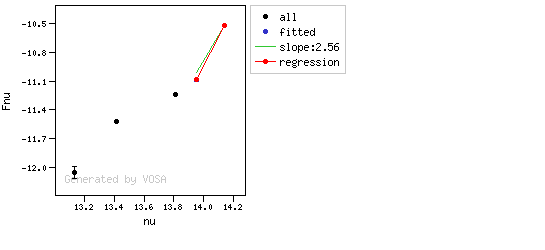
Points used for regression at WISE/WISE.W2: FilterID Wavelength Flux ΔFlux log(nu) log(nuFnu) e_log(nuFnu) weight
2MASS/2MASS.Ks 21590 1.3987756851941E-15 2.4478080312896E-17 14.1426 -10.52 0.0076 17313
WISE/WISE.W1 33526 2.4473412676635E-16 7.3027728843144E-18 13.9514 -11.0859 0.0129592 5954.49
WISE/WISE.W2 46028 1.2557903316284E-16 2.313251278027E-18 13.8138 -11.2381 0.008 15625
b + σ(b) = 2.24699 < 2.56 ⇒ excess?
yL= -11.3616
(yobs-yL)/σ(y) = 15.4485 ⇒ excess?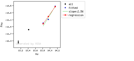
Points used for regression at WISE/WISE.W3: FilterID Wavelength Flux ΔFlux log(nu) log(nuFnu) e_log(nuFnu) weight
2MASS/2MASS.Ks 21590 1.3987756851941E-15 2.4478080312896E-17 14.1426 -10.52 0.0076 17313
WISE/WISE.W1 33526 2.4473412676635E-16 7.3027728843144E-18 13.9514 -11.0859 0.0129592 5954.49
WISE/WISE.W3 115608 2.6104843027125E-17 5.770427751284E-19 13.4138 -11.5203 0.0096 10850.7
b + σ(b) = 1.35201 < 2.56 ⇒ excess?
yL= -12.3856
(yobs-yL)/σ(y) = 90.1323 ⇒ excess?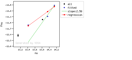
Points used for regression at WISE/WISE.W4: FilterID Wavelength Flux ΔFlux log(nu) log(nuFnu) e_log(nuFnu) weight
2MASS/2MASS.Ks
21590
1.3987756851941E-15
2.4478080312896E-17
14.1426
-10.52
0.0076
17313
WISE/WISE.W1
33526
2.4473412676635E-16
7.3027728843144E-18
13.9514
-11.0859
0.0129592
5954.49
WISE/WISE.W4
220883
4.0506648798552E-18
5.5962003414414E-19
13.1327
-12.0483
0.06
277.778
b + σ(b) = 2.08151 < 2.56 ⇒ excess?
yL= -13.1054
(yobs-yL)/σ(y) = 17.6176 ⇒ excess?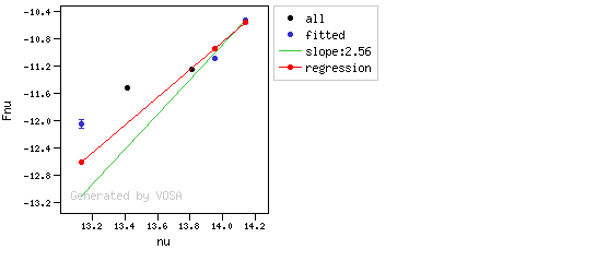
WISE/WISE.W4: b - σ(b) = 1.98338 < 2.56
And at least one of the last two points meets the final criterium.2.- Only one "suspicious" point.
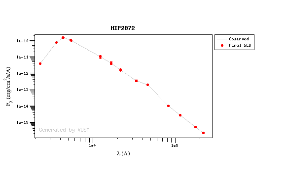
np FilterID Wavelength Flux ΔFlux log(nu) log(nuFnu) e_log(nuFnu) weight exc a b σa σb nsig b+σb<2.56
nsig>3
•
0 2MASS/2MASS.Ks 21590 1.5694521322167E-12 4.2209149938899E-13 14.1426 -7.47 0.1168 73.3017 --- --- --- --- --- --- --- --- •
1 WISE/WISE.W1 33526 3.3657687844505E-13 3.9369842670065E-14 13.9514 -7.94753 0.0508 387.501 --- -42.8051 2.49849 9.31766 0.666403 0.231413 --- --- •
2 WISE/WISE.W2 46028 1.9431983592016E-13 1.5033915370751E-14 13.8138 -8.04846 0.0336 885.771 1 -26.7667 1.35378 4.21877 0.30413 7.83299 yes yes •
3 AKARI/IRC.S9W 82283.5545614 9.5951888798357E-15 1.13796194837E-16 13.5615 -9.10263 0.00515061 37694.9 --- -48.6621 2.91705 1.49198 0.109974 -28.1752 --- --- •
4 WISE/WISE.W3 115608 2.5160605366691E-15 3.2443283514907E-17 13.4138 -9.53629 0.0056 31887.8 --- -48.8794 2.93305 0.610999 0.0452683 -35.8446 --- --- •
5 AKARI/IRC.L18W 176094.903177 5.0301502726085E-16 2.3106014129414E-17 13.2311 -10.0527 0.0199493 2512.71 --- -48.623 2.91408 0.525192 0.0389372 -12.494 --- --- •
6 WISE/WISE.W4 220883 2.2076301392736E-16 3.8632747496472E-18 13.1327 -10.3119 0.0076 17313 --- -47.4767 2.82926 0.272648 0.0203159 -33.7557 --- --- Details, point by point
Points used for regression at WISE/WISE.W1: FilterID Wavelength Flux ΔFlux log(nu) log(nuFnu) e_log(nuFnu) weight
2MASS/2MASS.Ks
21590
1.5694521322167E-12
4.2209149938899E-13
14.1426
-7.47
0.1168
73.3017
WISE/WISE.W1
33526
3.3657687844505E-13
3.9369842670065E-14
13.9514
-7.94753
0.0508
387.501
b + σ(b) = 3.1649 > 2.56 ⇒ NO excess
yL= -7.95929
(yobs-yL)/σ(y) = 0.231413 ⇒ NO excess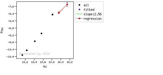
Points used for regression at WISE/WISE.W2: FilterID Wavelength Flux ΔFlux log(nu) log(nuFnu) e_log(nuFnu) weight
2MASS/2MASS.Ks
21590
1.5694521322167E-12
4.2209149938899E-13
14.1426
-7.47
0.1168
73.3017
WISE/WISE.W1
33526
3.3657687844505E-13
3.9369842670065E-14
13.9514
-7.94753
0.0508
387.501
WISE/WISE.W2
46028
1.9431983592016E-13
1.5033915370751E-14
13.8138
-8.04846
0.0336
885.771
b + σ(b) = 1.65791 < 2.56 ⇒ excess?
yL= -8.31165
(yobs-yL)/σ(y) = 7.83299 ⇒ excess?
Points used for regression at AKARI/IRC.S9W: FilterID Wavelength Flux ΔFlux log(nu) log(nuFnu) e_log(nuFnu) weight
2MASS/2MASS.Ks
21590
1.5694521322167E-12
4.2209149938899E-13
14.1426
-7.47
0.1168
73.3017
WISE/WISE.W1
33526
3.3657687844505E-13
3.9369842670065E-14
13.9514
-7.94753
0.0508
387.501
AKARI/IRC.S9W
82283.5545614
9.5951888798357E-15
1.13796194837E-16
13.5615
-9.10263
0.00515061
37694.9
b + σ(b) = 3.02702 > 2.56 ⇒ NO excess
yL= -8.95751
(yobs-yL)/σ(y) = -28.1752 ⇒ NO excess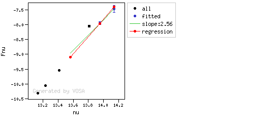
Points used for regression at WISE/WISE.W3: FilterID Wavelength Flux ΔFlux log(nu) log(nuFnu) e_log(nuFnu) weight
2MASS/2MASS.Ks
21590
1.5694521322167E-12
4.2209149938899E-13
14.1426
-7.47
0.1168
73.3017
WISE/WISE.W1
33526
3.3657687844505E-13
3.9369842670065E-14
13.9514
-7.94753
0.0508
387.501
AKARI/IRC.S9W
82283.5545614
9.5951888798357E-15
1.13796194837E-16
13.5615
-9.10263
0.00515061
37694.9
WISE/WISE.W3
115608
2.5160605366691E-15
3.2443283514907E-17
13.4138
-9.53629
0.0056
31887.8
b + σ(b) = 2.97832 > 2.56 ⇒ NO excess
yL= -9.33556
(yobs-yL)/σ(y) = -35.8446 ⇒ NO excess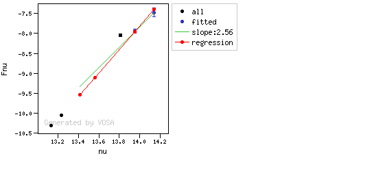
Points used for regression at AKARI/IRC.L18W: FilterID Wavelength Flux ΔFlux log(nu) log(nuFnu) e_log(nuFnu) weight
2MASS/2MASS.Ks
21590
1.5694521322167E-12
4.2209149938899E-13
14.1426
-7.47
0.1168
73.3017
WISE/WISE.W1
33526
3.3657687844505E-13
3.9369842670065E-14
13.9514
-7.94753
0.0508
387.501
AKARI/IRC.S9W
82283.5545614
9.5951888798357E-15
1.13796194837E-16
13.5615
-9.10263
0.00515061
37694.9
WISE/WISE.W3
115608
2.5160605366691E-15
3.2443283514907E-17
13.4138
-9.53629
0.0056
31887.8
AKARI/IRC.L18W
176094.903177
5.0301502726085E-16
2.3106014129414E-17
13.2311
-10.0527
0.0199493
2512.71
b + σ(b) = 2.95302 > 2.56 ⇒ NO excess
yL= -9.80342
(yobs-yL)/σ(y) = -12.494 ⇒ NO excess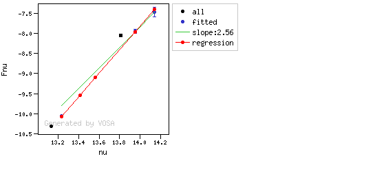
Points used for regression at WISE/WISE.W4: FilterID Wavelength Flux ΔFlux log(nu) log(nuFnu) e_log(nuFnu) weight
2MASS/2MASS.Ks
21590
1.5694521322167E-12
4.2209149938899E-13
14.1426
-7.47
0.1168
73.3017
WISE/WISE.W1
33526
3.3657687844505E-13
3.9369842670065E-14
13.9514
-7.94753
0.0508
387.501
AKARI/IRC.S9W
82283.5545614
9.5951888798357E-15
1.13796194837E-16
13.5615
-9.10263
0.00515061
37694.9
WISE/WISE.W3
115608
2.5160605366691E-15
3.2443283514907E-17
13.4138
-9.53629
0.0056
31887.8
AKARI/IRC.L18W
176094.903177
5.0301502726085E-16
2.3106014129414E-17
13.2311
-10.0527
0.0199493
2512.71
WISE/WISE.W4
220883
2.2076301392736E-16
3.8632747496472E-18
13.1327
-10.3119
0.0076
17313
b + σ(b) = 2.84957 > 2.56 ⇒ NO excess
yL= -10.0554
(yobs-yL)/σ(y) = -33.7557 ⇒ NO excess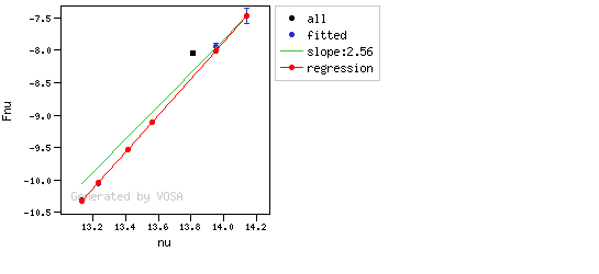
3.- Final check fails.
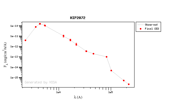
np FilterID Wavelength Flux ΔFlux log(nu) log(nuFnu) e_log(nuFnu) weight exc a b σa σb nsig b+σb<2.56
nsig>3
•
0 2MASS/2MASS.Ks 21590 1.5694521322167E-12 4.2209149938899E-13 14.1426 -7.47 0.1168 73.3017 --- --- --- --- --- --- --- --- •
1 WISE/WISE.W1 33526 3.3657687844505E-13 3.9369842670065E-14 13.9514 -7.94753 0.0508 387.501 --- -42.8051 2.49849 9.31766 0.666403 0.231413 --- --- •
2 WISE/WISE.W2 46028 1.9431983592016E-13 1.5033915370751E-14 13.8138 -8.04846 0.0336 885.771 1 -26.7667 1.35378 4.21877 0.30413 7.83299 yes yes •
3 AKARI/IRC.S9W 82283.5545614 9.5951888798357E-14 1.13796194837E-16 13.5615 -8.10263 0.000515061 3.76949e+6 1 -16.2689 0.602166 1.48272 0.109332 1659.77 yes yes •
4 IRAS/IRAS.12mu 101464.582668 4.571844088105E-15 2.9776333734753E-16 13.4705 -9.33359 0.0282855 1249.89 --- -47.7263 2.85022 1.4324 0.105245 -5.05971 --- --- •
5 AKARI/IRC.L18W 176094.903177 5.0301502726085E-16 2.3106014129414E-17 13.2311 -10.0527 0.0199493 2512.71 --- -48.5768 2.91209 0.873078 0.0652236 -12.494 --- --- •
6 WISE/WISE.W4 220883 2.2076301392736E-16 3.8632747496472E-18 13.1327 -10.3119 0.0076 17313 --- -48.0225 2.87135 0.621932 0.0471779 -33.7557 --- --- Details, point by point
Points used for regression at WISE/WISE.W1: FilterID Wavelength Flux ΔFlux log(nu) log(nuFnu) e_log(nuFnu) weight
2MASS/2MASS.Ks
21590
1.5694521322167E-12
4.2209149938899E-13
14.1426
-7.47
0.1168
73.3017
WISE/WISE.W1
33526
3.3657687844505E-13
3.9369842670065E-14
13.9514
-7.94753
0.0508
387.501
b + σ(b) = 3.1649 > 2.56 ⇒ NO excess
yL= -7.95929
(yobs-yL)/σ(y) = 0.231413 ⇒ NO excess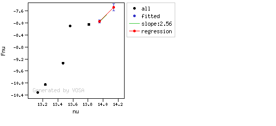
Points used for regression at WISE/WISE.W2: FilterID Wavelength Flux ΔFlux log(nu) log(nuFnu) e_log(nuFnu) weight
2MASS/2MASS.Ks
21590
1.5694521322167E-12
4.2209149938899E-13
14.1426
-7.47
0.1168
73.3017
WISE/WISE.W1
33526
3.3657687844505E-13
3.9369842670065E-14
13.9514
-7.94753
0.0508
387.501
WISE/WISE.W2
46028
1.9431983592016E-13
1.5033915370751E-14
13.8138
-8.04846
0.0336
885.771
b + σ(b) = 1.65791 < 2.56 ⇒ excess?
yL= -8.31165
(yobs-yL)/σ(y) = 7.83299 ⇒ excess?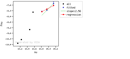
Points used for regression at AKARI/IRC.S9W: FilterID Wavelength Flux ΔFlux log(nu) log(nuFnu) e_log(nuFnu) weight
2MASS/2MASS.Ks
21590
1.5694521322167E-12
4.2209149938899E-13
14.1426
-7.47
0.1168
73.3017
WISE/WISE.W1
33526
3.3657687844505E-13
3.9369842670065E-14
13.9514
-7.94753
0.0508
387.501
AKARI/IRC.S9W
82283.5545614
9.5951888798357E-14
1.13796194837E-16
13.5615
-8.10263
0.000515061
3.76949e+6
b + σ(b) = 0.711498 < 2.56 ⇒ excess?
yL= -8.95751
(yobs-yL)/σ(y) = 1659.77 ⇒ excess?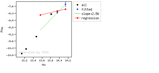
Points used for regression at IRAS/IRAS.12mu: FilterID Wavelength Flux ΔFlux log(nu) log(nuFnu) e_log(nuFnu) weight
2MASS/2MASS.Ks
21590
1.5694521322167E-12
4.2209149938899E-13
14.1426
-7.47
0.1168
73.3017
WISE/WISE.W1
33526
3.3657687844505E-13
3.9369842670065E-14
13.9514
-7.94753
0.0508
387.501
IRAS/IRAS.12mu
101464.582668
4.571844088105E-15
2.9776333734753E-16
13.4705
-9.33359
0.0282855
1249.89
b + σ(b) = 2.95547 > 2.56 ⇒ NO excess
yL= -9.19048
(yobs-yL)/σ(y) = -5.05971 ⇒ NO excess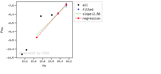
Points used for regression at AKARI/IRC.L18W: FilterID Wavelength Flux ΔFlux log(nu) log(nuFnu) e_log(nuFnu) weight
2MASS/2MASS.Ks
21590
1.5694521322167E-12
4.2209149938899E-13
14.1426
-7.47
0.1168
73.3017
WISE/WISE.W1
33526
3.3657687844505E-13
3.9369842670065E-14
13.9514
-7.94753
0.0508
387.501
IRAS/IRAS.12mu
101464.582668
4.571844088105E-15
2.9776333734753E-16
13.4705
-9.33359
0.0282855
1249.89
AKARI/IRC.L18W
176094.903177
5.0301502726085E-16
2.3106014129414E-17
13.2311
-10.0527
0.0199493
2512.71
b + σ(b) = 2.97731 > 2.56 ⇒ NO excess
yL= -9.80342
(yobs-yL)/σ(y) = -12.494 ⇒ NO excess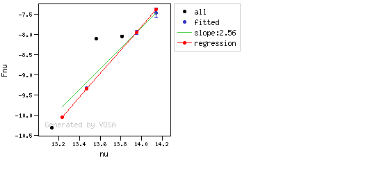
Points used for regression at WISE/WISE.W4: FilterID Wavelength Flux ΔFlux log(nu) log(nuFnu) e_log(nuFnu) weight
2MASS/2MASS.Ks
21590
1.5694521322167E-12
4.2209149938899E-13
14.1426
-7.47
0.1168
73.3017
WISE/WISE.W1
33526
3.3657687844505E-13
3.9369842670065E-14
13.9514
-7.94753
0.0508
387.501
IRAS/IRAS.12mu
101464.582668
4.571844088105E-15
2.9776333734753E-16
13.4705
-9.33359
0.0282855
1249.89
AKARI/IRC.L18W
176094.903177
5.0301502726085E-16
2.3106014129414E-17
13.2311
-10.0527
0.0199493
2512.71
WISE/WISE.W4
220883
2.2076301392736E-16
3.8632747496472E-18
13.1327
-10.3119
0.0076
17313
b + σ(b) = 2.91852 > 2.56 ⇒ NO excess
yL= -10.0554
(yobs-yL)/σ(y) = -33.7557 ⇒ NO excess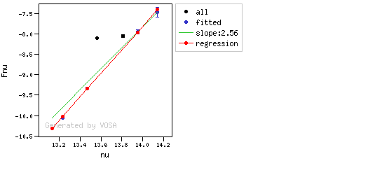
WISE/WISE.W4: b - σ(b) = 2.82417 > 2.56
But none of the last two points meets the final criterium.4.- Excess only in last point.
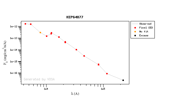
np FilterID Wavelength Flux ΔFlux log(nu) log(nuFnu) e_log(nuFnu) weight exc a b σa σb nsig b+σb<2.56
nsig>3
•
0 2MASS/2MASS.Ks 21590 4.6617402846124E-14 1.331022657158E-15 14.1426 -8.9972 0.0124 6503.64 --- --- --- --- --- --- --- --- •
1 WISE/WISE.W1 33526 1.0024997622146E-14 2.3083410082054E-16 13.9514 -9.47353 0.01 10000 --- -44.2435 2.49221 1.1691 0.083346 1.29558 --- --- •
2 WISE/WISE.W2 46028 2.9115022836668E-15 4.8268668647443E-17 13.8138 -9.87286 0.0072 19290.1 --- -46.9843 2.68704 0.594682 0.0427443 -4.72384 --- --- •
3 AKARI/IRC.S9W 82283.5545614 5.2381672565047E-16 7.483096080721E-17 13.5615 -10.3655 0.0620421 259.793 --- -46.5955 2.65918 0.578079 0.0415584 1.92138 --- --- •
4 WISE/WISE.W3 115608 8.8129455335059E-17 1.5422343328222E-18 13.4138 -10.9919 0.0076 17313 --- -48.146 2.77039 0.234038 0.0170197 -16.9907 --- --- •
5 WISE/WISE.W4 220883 2.3074182037759E-17 8.0758006741624E-19 13.1327 -11.2927 0.0152 4328.25 1 -44.9115 2.53692 0.194382 0.0141827 19.0695 yes yes Details, point by point
Points used for regression at WISE/WISE.W1: FilterID Wavelength Flux ΔFlux log(nu) log(nuFnu) e_log(nuFnu) weight
2MASS/2MASS.Ks
21590
4.6617402846124E-14
1.331022657158E-15
14.1426
-8.9972
0.0124
6503.64
WISE/WISE.W1
33526
1.0024997622146E-14
2.3083410082054E-16
13.9514
-9.47353
0.01
10000
b + σ(b) = 2.57556 > 2.56 ⇒ NO excess
yL= -9.48649
(yobs-yL)/σ(y) = 1.29558 ⇒ NO excess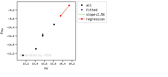
Points used for regression at WISE/WISE.W2: FilterID Wavelength Flux ΔFlux log(nu) log(nuFnu) e_log(nuFnu) weight
2MASS/2MASS.Ks
21590
4.6617402846124E-14
1.331022657158E-15
14.1426
-8.9972
0.0124
6503.64
WISE/WISE.W1
33526
1.0024997622146E-14
2.3083410082054E-16
13.9514
-9.47353
0.01
10000
WISE/WISE.W2
46028
2.9115022836668E-15
4.8268668647443E-17
13.8138
-9.87286
0.0072
19290.1
b + σ(b) = 2.72979 > 2.56 ⇒ NO excess
yL= -9.83885
(yobs-yL)/σ(y) = -4.72384 ⇒ NO excess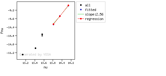
Points used for regression at AKARI/IRC.S9W: FilterID Wavelength Flux ΔFlux log(nu) log(nuFnu) e_log(nuFnu) weight
2MASS/2MASS.Ks
21590
4.6617402846124E-14
1.331022657158E-15
14.1426
-8.9972
0.0124
6503.64
WISE/WISE.W1
33526
1.0024997622146E-14
2.3083410082054E-16
13.9514
-9.47353
0.01
10000
WISE/WISE.W2
46028
2.9115022836668E-15
4.8268668647443E-17
13.8138
-9.87286
0.0072
19290.1
AKARI/IRC.S9W
82283.5545614
5.2381672565047E-16
7.483096080721E-17
13.5615
-10.3655
0.0620421
259.793
b + σ(b) = 2.70074 > 2.56 ⇒ NO excess
yL= -10.4847
(yobs-yL)/σ(y) = 1.92138 ⇒ NO excess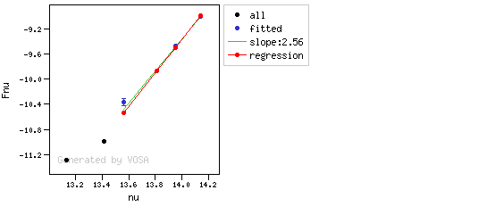
Points used for regression at WISE/WISE.W3: FilterID Wavelength Flux ΔFlux log(nu) log(nuFnu) e_log(nuFnu) weight
2MASS/2MASS.Ks
21590
4.6617402846124E-14
1.331022657158E-15
14.1426
-8.9972
0.0124
6503.64
WISE/WISE.W1
33526
1.0024997622146E-14
2.3083410082054E-16
13.9514
-9.47353
0.01
10000
WISE/WISE.W2
46028
2.9115022836668E-15
4.8268668647443E-17
13.8138
-9.87286
0.0072
19290.1
AKARI/IRC.S9W
82283.5545614
5.2381672565047E-16
7.483096080721E-17
13.5615
-10.3655
0.0620421
259.793
WISE/WISE.W3
115608
8.8129455335059E-17
1.5422343328222E-18
13.4138
-10.9919
0.0076
17313
b + σ(b) = 2.78741 > 2.56 ⇒ NO excess
yL= -10.8628
(yobs-yL)/σ(y) = -16.9907 ⇒ NO excess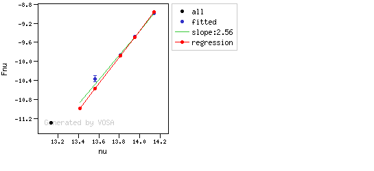
Points used for regression at WISE/WISE.W4: FilterID Wavelength Flux ΔFlux log(nu) log(nuFnu) e_log(nuFnu) weight
2MASS/2MASS.Ks
21590
4.6617402846124E-14
1.331022657158E-15
14.1426
-8.9972
0.0124
6503.64
WISE/WISE.W1
33526
1.0024997622146E-14
2.3083410082054E-16
13.9514
-9.47353
0.01
10000
WISE/WISE.W2
46028
2.9115022836668E-15
4.8268668647443E-17
13.8138
-9.87286
0.0072
19290.1
AKARI/IRC.S9W
82283.5545614
5.2381672565047E-16
7.483096080721E-17
13.5615
-10.3655
0.0620421
259.793
WISE/WISE.W3
115608
8.8129455335059E-17
1.5422343328222E-18
13.4138
-10.9919
0.0076
17313
WISE/WISE.W4
220883
2.3074182037759E-17
8.0758006741624E-19
13.1327
-11.2927
0.0152
4328.25
b + σ(b) = 2.5511 < 2.56 ⇒ excess?
yL= -11.5826
(yobs-yL)/σ(y) = 19.0695 ⇒ excess?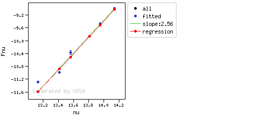
Appendix B: Total flux calculation example
lambda width start end flux error 3447 372 3261 3633 1.87e-12 2.33e-14 3570 657 3242 3899 5.98e-12 8.15e-13 4110 223 3998 4222 8.70e-12 5.40e-14 4280 708 3925 4634 9.48e-12 8.44e-14 4297 843 3875 4718 1.00e-11 7.33e-13 4378 972 3891 4864 9.77e-12 1.50e-12 4640 1158 4061 5219 9.60e-12 4.78e-14 4663 202 4562 4764 1.06e-11 2.50e-14 5340 1005 4837 5842 9.38e-12 6.66e-14 5394 870 4959 5829 7.31e-12 1.50e-13 5466 889 5021 5910 8.30e-12 1.44e-12 5472 253 5345 5599 8.63e-12 1.57e-14 5857 4203 3755 7959 6.89e-12 1.23e-12 6122 1111 5566 6677 5.79e-12 1.99e-13 7439 1044 6917 7961 4.60e-12 6.02e-13 12350 1624 11537 13162 1.51e-12 2.45e-14 16620 2509 15365 17874 6.85e-13 1.34e-14 21590 2618 20280 22899 2.66e-13 4.19e-15 33526 6626 30212 36839 4.73e-14 5.03e-15 46028 10422 40816 51239 1.66e-14 8.67e-16 82283 41027 61769 102797 1.50e-15 2.92e-17 101464 60670 71129 131799 7.88e-16 9.19e-17 115608 55055 88080 143135 3.91e-16 5.28e-18 217265 100173 167178 267352 6.24e-17 1.48e-17 220883 41016 200374 241391 3.25e-17 1.19e-18 519887 305160 367307 672467 1.29e-17 2.96e-18 952971 332639 786651 1119290 4.52e-17 1.04e-17
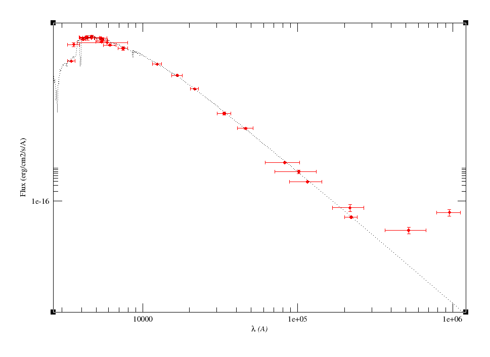
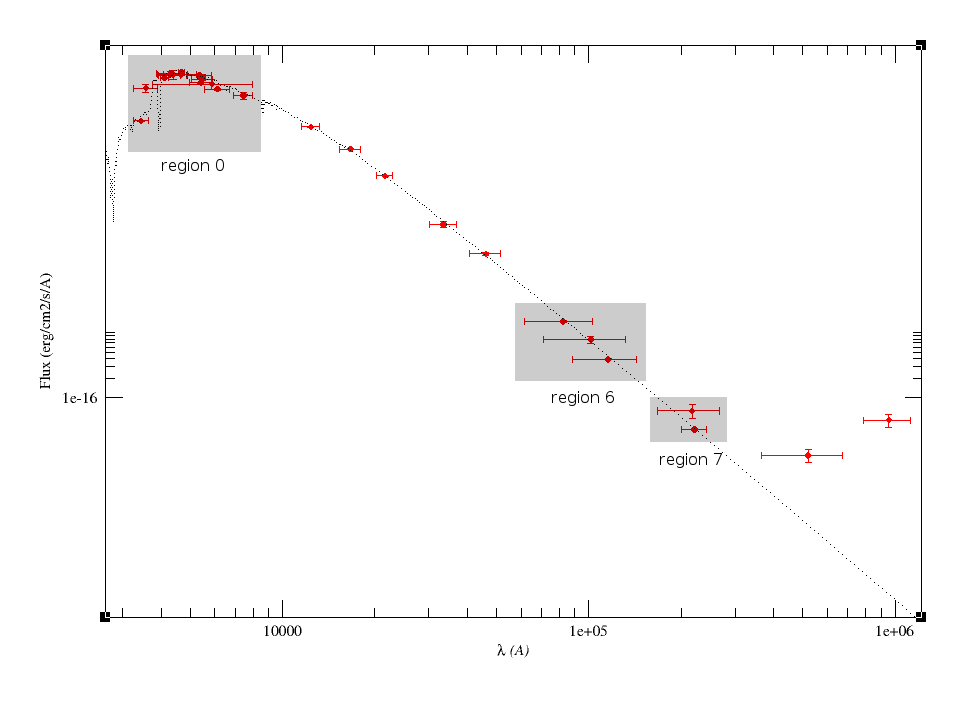
lambda width start end flux error 3447 372 3261 3633 1.87e-12 2.33e-14 3570 657 3242 3899 5.98e-12 8.15e-13 4110 223 3998 4222 8.70e-12 5.40e-14 4280 708 3925 4634 9.48e-12 8.44e-14 4297 843 3875 4718 1.00e-11 7.33e-13 4378 972 3891 4864 9.77e-12 1.50e-12 4640 1158 4061 5219 9.60e-12 4.78e-14 4663 202 4562 4764 1.06e-11 2.50e-14 5340 1005 4837 5842 9.38e-12 6.66e-14 5394 870 4959 5829 7.31e-12 1.50e-13 5466 889 5021 5910 8.30e-12 1.44e-12 5472 253 5345 5599 8.63e-12 1.57e-14 5857 4203 3755 7959 6.89e-12 1.23e-12 6122 1111 5566 6677 5.79e-12 1.99e-13 7439 1044 6917 7961 4.60e-12 6.02e-13 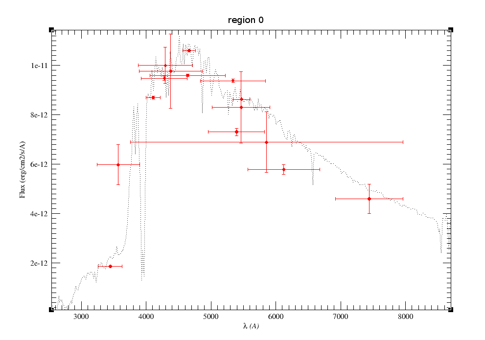
lambda width start end flux error 82283 41027 61769 102797 1.50e-15 2.92e-17 101464 60670 71129 131799 7.88e-16 9.19e-17 115608 55055 88080 143135 3.91e-16 5.28e-18 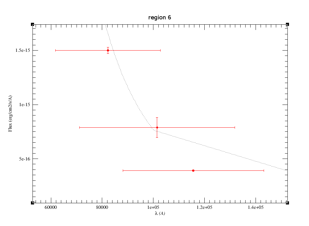
lambda width start end flux error 217265 100173 167178 267352 6.24e-17 1.48e-17 220883 41016 200374 241391 3.25e-17 1.19e-18 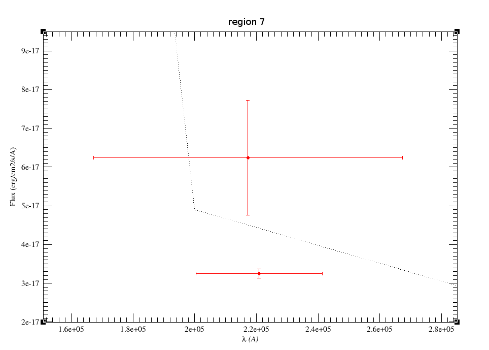
nreg tot $\lambda_{min}$ $\lambda_{max}$ len $\sum W_i$ over 0 15 3242 7961 4719 14516 3.076 1 1 11537 13162 1624 1624 1.000 2 1 15365 17874 2509 2509 1.000 3 1 20280 22899 2618 2618 1.000 4 1 30212 36839 6626 6626 1.000 5 1 40816 51239 10422 10422 1.000 6 3 61769 143135 81365 156753 1.927 7 2 167178 267352 100173 141190 1.409 8 1 367307 672467 305160 305160 1.000 9 1 786651 1119290 332639 332639 1.000
$$\int{\rm Md \cdot mod(\lambda) \ d\lambda} = 5.22 \ 10^{-8} $$
lambda width start end reg over flux error mod*md w*flx w*flx/over w*mod*md w*mod*md/over 3447 372 3261 3633 0 3.076 1.87e-12 2.33e-14 2.20e-12 6.98e-10 2.27e-10 8.20e-10 2.67e-10 3570 657 3242 3899 0 3.076 5.98e-12 8.15e-13 3.07e-12 3.93e-9 1.28e-9 2.02e-9 6.56e-10 4110 223 3998 4222 0 3.076 8.70e-12 5.40e-14 8.84e-12 1.95e-9 6.33e-10 1.98e-9 6.44e-10 4280 708 3925 4634 0 3.076 9.48e-12 8.44e-14 8.59e-12 6.72e-9 2.18e-9 6.08e-9 1.98e-9 4297 843 3875 4718 0 3.076 1.00e-11 7.33e-13 9.11e-12 8.45e-9 2.75e-9 7.68e-9 2.50e-9 4378 972 3891 4864 0 3.076 9.77e-12 1.50e-12 9.24e-12 9.50e-9 3.09e-9 8.99e-9 2.92e-9 4640 1158 4061 5219 0 3.076 9.60e-12 4.78e-14 9.58e-12 1.11e-8 3.62e-9 1.11e-8 3.61e-9 4663 202 4562 4764 0 3.076 1.06e-11 2.50e-14 1.05e-11 2.15e-9 6.98e-10 2.12e-9 6.90e-10 5340 1005 4837 5842 0 3.076 9.38e-12 6.66e-14 8.96e-12 9.43e-9 3.07e-9 9.01e-9 2.93e-9 5394 870 4959 5829 0 3.076 7.31e-12 1.50e-13 8.68e-12 6.37e-9 2.07e-9 7.56e-9 2.46e-9 5466 889 5021 5910 0 3.076 8.30e-12 1.44e-12 8.51e-12 7.38e-9 2.40e-9 7.58e-9 2.46e-9 5472 253 5345 5599 0 3.076 8.63e-12 1.57e-14 8.65e-12 2.19e-9 7.11e-10 2.19e-9 7.13e-10 5857 4203 3755 7959 0 3.076 6.89e-12 1.23e-12 6.40e-12 2.90e-8 9.42e-9 2.69e-8 8.75e-9 6122 1111 5566 6677 0 3.076 5.79e-12 1.99e-13 7.29e-12 6.43e-9 2.09e-9 8.10e-9 2.63e-9 7439 1044 6917 7961 0 3.076 4.60e-12 6.02e-13 4.98e-12 4.80e-9 1.56e-9 5.20e-9 1.69e-9 12350 1624 11537 13162 1 1.000 1.51e-12 2.45e-14 1.57e-12 2.45e-9 2.45e-9 2.55e-9 2.55e-9 16620 2509 15365 17874 2 1.000 6.85e-13 1.34e-14 6.74e-13 1.72e-9 1.72e-9 1.69e-9 1.69e-9 21590 2618 20280 22899 3 1.000 2.66e-13 4.19e-15 2.63e-13 6.98e-10 6.98e-10 6.90e-10 6.90e-10 33526 6626 30212 36839 4 1.000 4.73e-14 5.03e-15 5.26e-14 3.13e-10 3.13e-10 3.48e-10 3.48e-10 46028 10422 40816 51239 5 1.000 1.66e-14 8.67e-16 1.57e-14 1.73e-10 1.73e-10 1.64e-10 1.64e-10 82283 41027 61769 102797 6 1.927 1.50e-15 2.92e-17 1.37e-15 6.17e-11 3.20e-11 5.64e-11 2.93e-11 101464 60670 71129 131799 6 1.927 7.88e-16 9.19e-17 5.85e-16 4.78e-11 2.48e-11 3.55e-11 1.84e-11 115608 55055 88080 143135 6 1.927 3.91e-16 5.28e-18 4.25e-16 2.15e-11 1.12e-11 2.34e-11 1.21e-11 217265 100173 167178 267352 7 1.409 6.24e-17 1.48e-17 2.96e-17 6.25e-12 4.43e-12 2.96e-12 2.10e-12 220883 41016 200374 241391 7 1.409 3.25e-17 1.19e-18 3.20e-17 1.33e-12 9.47e-13 1.31e-12 9.31e-13 519887 305160 367307 672467 8 1.000 1.29e-17 2.96e-18 8.03e-19 3.93e-12 3.93e-12 2.45e-13 2.45e-13 952971 332639 786651 1119290 9 1.000 4.52e-17 1.04e-17 8.50e-20 1.51e-11 1.51e-11 2.83e-14 2.83e-14 reg Σ w*flx Σ w*mod*md Σ w*flx/over Σ w*mod*md/over 0 1.1e-7 1.07e-7 3.58e-8 3.49e-8 1 2.45e-9 2.55e-9 2.45e-9 2.55e-9 2 1.72e-9 1.69e-9 1.72e-9 1.69e-9 3 6.98e-10 6.9e-10 6.98e-10 6.9e-10 4 3.13e-10 3.48e-10 3.13e-10 3.48e-10 5 1.73e-10 1.64e-10 1.73e-10 1.64e-10 6 1.31e-10 1.15e-10 6.8e-11 5.98e-11 7 7.58e-12 4.27e-12 5.38e-12 3.03e-12 8 3.93e-12 2.45e-13 3.93e-12 2.45e-13 9 1.51e-11 2.83e-14 1.51e-11 2.83e-14 Σ 1.16e-7 1.13e-7 4.12e-8 4.04e-8 Ftot 5.49e-8 5.3e-8 Fobs 1.16e-7 4.12e-8 Fobs/Ftot 2.11 0.778 Appendix C: Quality information in VO Catalogs
2MASS All-Sky Point Source Catalog
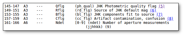
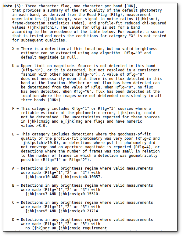
AKARI/FIS All-Sky Survey Point Source Catalogues (ISAS/JAXA, 2010)
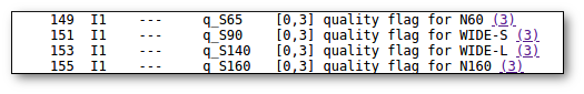
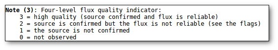
AKARI/IRC mid-IR all-sky Survey (ISAS/JAXA, 2010)

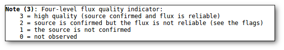
WISE

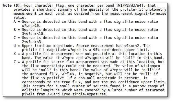
DENIS Catalogue


DARK ENERGY SURVEY, DR1
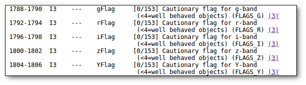

Galaxy Evolution Explorer [Galex-DR5 MIS]
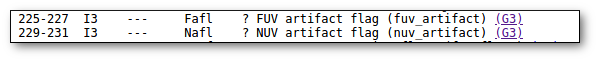
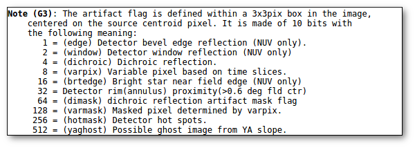
MSX6C Infrared Point Source Catalog
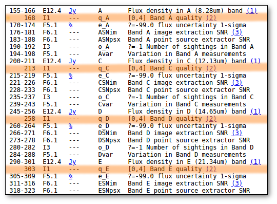
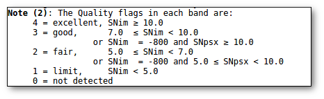
Pan-Starrs PS1 DR2
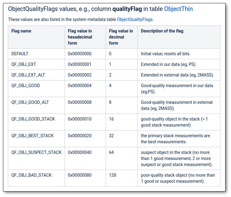
SDSS Catalogue, Release 12

UKIDSS Deep Extragalactic Survey DR10

UKIDSS Galactic Clusters Survey DR10

UKIDSS Galactic Plane Survey DR8

UKIDSS Large Area Survey DR10

UKIDSS Ultra Deep Survey DR10

VHS - VISTA Hemisphere Survey, DR6

VIDEO - VISTA Deep Extragalactic Observations Survey, DR5

VIKING - VISTA Kilo-Degree Infrared Galaxy Survey, DR4
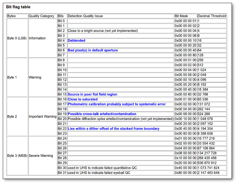
VMC - VISTA Magellanic Survey, DR4

VVV - VISTA Variables in the Via Lactea, DR4

VPHAS+ DR2