Total flux calculation exampleWe want to to calculate the total "observed flux" using the photometric values corresponding to different filters.
But we have observed photometric values corresponding to filters covering wavelength ranges that, often, overlap with each other.
We want to:
- First, discover what filters are overlaping with each other.
- Define wavelength regions with apreciable overlaping.
- Estimate the amount of overlaping in each of those regions.
- Estimate the total observed flux, suming up the contribution of each observation but weighted by the amount of overlaping in the corresponding region.
With this purpose:
- we use the filter effective width as an estimation of the wavelength range covered by each filter.
| lambda | width | start | end | flux | error |
| 3447 | 372 | 3261 | 3633 | 1.87e-12 | 2.33e-14 |
| 3570 | 657 | 3242 | 3899 | 5.98e-12 | 8.15e-13 |
| 4110 | 223 | 3998 | 4222 | 8.70e-12 | 5.40e-14 |
| 4280 | 708 | 3925 | 4634 | 9.48e-12 | 8.44e-14 |
| 4297 | 843 | 3875 | 4718 | 1.00e-11 | 7.33e-13 |
| 4378 | 972 | 3891 | 4864 | 9.77e-12 | 1.50e-12 |
| 4640 | 1158 | 4061 | 5219 | 9.60e-12 | 4.78e-14 |
| 4663 | 202 | 4562 | 4764 | 1.06e-11 | 2.50e-14 |
| 5340 | 1005 | 4837 | 5842 | 9.38e-12 | 6.66e-14 |
| 5394 | 870 | 4959 | 5829 | 7.31e-12 | 1.50e-13 |
| 5466 | 889 | 5021 | 5910 | 8.30e-12 | 1.44e-12 |
| 5472 | 253 | 5345 | 5599 | 8.63e-12 | 1.57e-14 |
| 5857 | 4203 | 3755 | 7959 | 6.89e-12 | 1.23e-12 |
| 6122 | 1111 | 5566 | 6677 | 5.79e-12 | 1.99e-13 |
| 7439 | 1044 | 6917 | 7961 | 4.60e-12 | 6.02e-13 |
| 12350 | 1624 | 11537 | 13162 | 1.51e-12 | 2.45e-14 |
| 16620 | 2509 | 15365 | 17874 | 6.85e-13 | 1.34e-14 |
| 21590 | 2618 | 20280 | 22899 | 2.66e-13 | 4.19e-15 |
| 33526 | 6626 | 30212 | 36839 | 4.73e-14 | 5.03e-15 |
| 46028 | 10422 | 40816 | 51239 | 1.66e-14 | 8.67e-16 |
| 82283 | 41027 | 61769 | 102797 | 1.50e-15 | 2.92e-17 |
| 101464 | 60670 | 71129 | 131799 | 7.88e-16 | 9.19e-17 |
| 115608 | 55055 | 88080 | 143135 | 3.91e-16 | 5.28e-18 |
| 217265 | 100173 | 167178 | 267352 | 6.24e-17 | 1.48e-17 |
| 220883 | 41016 | 200374 | 241391 | 3.25e-17 | 1.19e-18 |
| 519887 | 305160 | 367307 | 672467 | 1.29e-17 | 2.96e-18 |
| 952971 | 332639 | 786651 | 1119290 | 4.52e-17 | 1.04e-17 |
|

|
- Using this, we find the regions where we have continuous filter coverage.
To do this, we define different regions when the last filter in one region ends before the starting point of the first filter in the following region.
In this case, we find 10 different regions:
- 7 of them contain only one filter and they can be considered "simple regions" with no overlaping.
- 3 of them contain 2 or more overlaping filters.
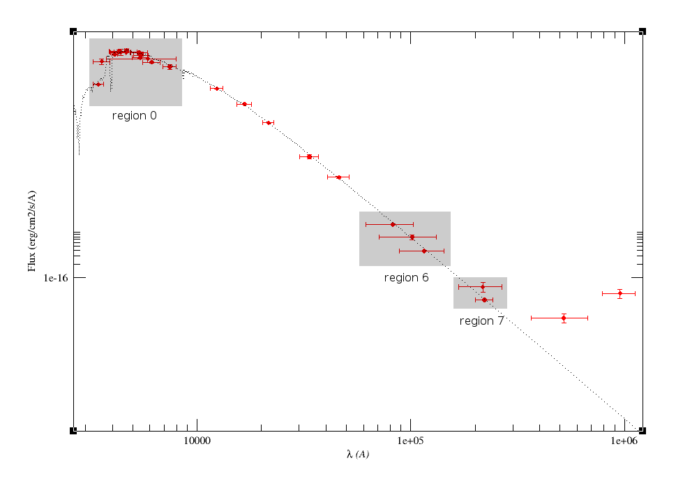
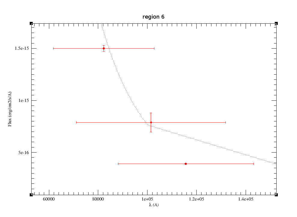
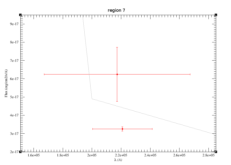
We see, with more detail, the three complex regions containing more than one overlaping filters:
|
| lambda | width | start | end | flux | error |
| 3447 | 372 | 3261 | 3633 | 1.87e-12 | 2.33e-14 |
| 3570 | 657 | 3242 | 3899 | 5.98e-12 | 8.15e-13 |
| 4110 | 223 | 3998 | 4222 | 8.70e-12 | 5.40e-14 |
| 4280 | 708 | 3925 | 4634 | 9.48e-12 | 8.44e-14 |
| 4297 | 843 | 3875 | 4718 | 1.00e-11 | 7.33e-13 |
| 4378 | 972 | 3891 | 4864 | 9.77e-12 | 1.50e-12 |
| 4640 | 1158 | 4061 | 5219 | 9.60e-12 | 4.78e-14 |
| 4663 | 202 | 4562 | 4764 | 1.06e-11 | 2.50e-14 |
| 5340 | 1005 | 4837 | 5842 | 9.38e-12 | 6.66e-14 |
| 5394 | 870 | 4959 | 5829 | 7.31e-12 | 1.50e-13 |
| 5466 | 889 | 5021 | 5910 | 8.30e-12 | 1.44e-12 |
| 5472 | 253 | 5345 | 5599 | 8.63e-12 | 1.57e-14 |
| 5857 | 4203 | 3755 | 7959 | 6.89e-12 | 1.23e-12 |
| 6122 | 1111 | 5566 | 6677 | 5.79e-12 | 1.99e-13 |
| 7439 | 1044 | 6917 | 7961 | 4.60e-12 | 6.02e-13 |
|
 |
|
| lambda | width | start | end | flux | error |
| 82283 | 41027 | 61769 | 102797 | 1.50e-15 | 2.92e-17 |
| 101464 | 60670 | 71129 | 131799 | 7.88e-16 | 9.19e-17 |
| 115608 | 55055 | 88080 | 143135 | 3.91e-16 | 5.28e-18 |
|
 |
|
| lambda | width | start | end | flux | error |
| 217265 | 100173 | 167178 | 267352 | 6.24e-17 | 1.48e-17 |
| 220883 | 41016 | 200374 | 241391 | 3.25e-17 | 1.19e-18 |
|
 |
- For each region, we define the amount of overlaping as the ratio between the sum of lengths of the filters in the region and the lenght of the region.
$$ {\rm over} = \frac{\sum {\rm W}_i}{\rm (\lambda_{\rm max} - \lambda_{\rm min})}$$
Regions:
| nreg | tot | $\lambda_{min}$ | $\lambda_{max}$ | len | $\sum W_i$ | over |
| 0 | 15 | 3242 | 7961 | 4719 | 14516 | 3.076 |
| 1 | 1 | 11537 | 13162 | 1624 | 1624 | 1.000 |
| 2 | 1 | 15365 | 17874 | 2509 | 2509 | 1.000 |
| 3 | 1 | 20280 | 22899 | 2618 | 2618 | 1.000 |
| 4 | 1 | 30212 | 36839 | 6626 | 6626 | 1.000 |
| 5 | 1 | 40816 | 51239 | 10422 | 10422 | 1.000 |
| 6 | 3 | 61769 | 143135 | 81365 | 156753 | 1.927 |
| 7 | 2 | 167178 | 267352 | 100173 | 141190 | 1.409 |
| 8 | 1 | 367307 | 672467 | 305160 | 305160 | 1.000 |
| 9 | 1 | 786651 | 1119290 | 332639 | 332639 | 1.000 |
- Then, to calculate the total observed flux, we have to weight the contribution from each observed photometric point, dividing it by the amount of overlaping in the correponding region.
$$ {\rm Fobs} = \frac{\sum {\rm F_{o,i}} \cdot {\rm W_{eff,i}}}{ {\rm Over_i}} $$
We also do the equivalent calculation for the model fluxes corresponding to the observations:
$$ {\rm Fmod} = \frac{\sum {\rm Md \cdot F_{M,i}} \cdot {\rm W_{eff,i}}}{ {\rm Over_i}} $$
The total flux is the total flux of the model plus the estimated observed flux minus the estimated model flux corresponding to the observations:
$${\rm Ftot} = \int{\rm Md \cdot mod(\lambda) \ d\lambda} \ + {\rm Fobs} - {\rm Fmod} $$
In this particular case, we have:
- Kurucz model
- Teff = 6250 K
- logg = 0.50
- meta = 0.50
- Md=6.239e-18
$$\int{\rm Md \cdot mod(\lambda) \ d\lambda} = 5.22 \ 10^{-8} $$
- If we make the calculations filter by filter, we get very different results if we take into account the overlaping.
The partial numbers for each filter are:
| lambda | width | start | end | reg | over | flux | error | mod*md | w*flx | w*flx/over | w*mod*md | w*mod*md/over |
| 3447 | 372 | 3261 | 3633 | 0 | 3.076 | 1.87e-12 | 2.33e-14 | 2.20e-12 | 6.98e-10 | 2.27e-10 | 8.20e-10 | 2.67e-10 |
| 3570 | 657 | 3242 | 3899 | 0 | 3.076 | 5.98e-12 | 8.15e-13 | 3.07e-12 | 3.93e-9 | 1.28e-9 | 2.02e-9 | 6.56e-10 |
| 4110 | 223 | 3998 | 4222 | 0 | 3.076 | 8.70e-12 | 5.40e-14 | 8.84e-12 | 1.95e-9 | 6.33e-10 | 1.98e-9 | 6.44e-10 |
| 4280 | 708 | 3925 | 4634 | 0 | 3.076 | 9.48e-12 | 8.44e-14 | 8.59e-12 | 6.72e-9 | 2.18e-9 | 6.08e-9 | 1.98e-9 |
| 4297 | 843 | 3875 | 4718 | 0 | 3.076 | 1.00e-11 | 7.33e-13 | 9.11e-12 | 8.45e-9 | 2.75e-9 | 7.68e-9 | 2.50e-9 |
| 4378 | 972 | 3891 | 4864 | 0 | 3.076 | 9.77e-12 | 1.50e-12 | 9.24e-12 | 9.50e-9 | 3.09e-9 | 8.99e-9 | 2.92e-9 |
| 4640 | 1158 | 4061 | 5219 | 0 | 3.076 | 9.60e-12 | 4.78e-14 | 9.58e-12 | 1.11e-8 | 3.62e-9 | 1.11e-8 | 3.61e-9 |
| 4663 | 202 | 4562 | 4764 | 0 | 3.076 | 1.06e-11 | 2.50e-14 | 1.05e-11 | 2.15e-9 | 6.98e-10 | 2.12e-9 | 6.90e-10 |
| 5340 | 1005 | 4837 | 5842 | 0 | 3.076 | 9.38e-12 | 6.66e-14 | 8.96e-12 | 9.43e-9 | 3.07e-9 | 9.01e-9 | 2.93e-9 |
| 5394 | 870 | 4959 | 5829 | 0 | 3.076 | 7.31e-12 | 1.50e-13 | 8.68e-12 | 6.37e-9 | 2.07e-9 | 7.56e-9 | 2.46e-9 |
| 5466 | 889 | 5021 | 5910 | 0 | 3.076 | 8.30e-12 | 1.44e-12 | 8.51e-12 | 7.38e-9 | 2.40e-9 | 7.58e-9 | 2.46e-9 |
| 5472 | 253 | 5345 | 5599 | 0 | 3.076 | 8.63e-12 | 1.57e-14 | 8.65e-12 | 2.19e-9 | 7.11e-10 | 2.19e-9 | 7.13e-10 |
| 5857 | 4203 | 3755 | 7959 | 0 | 3.076 | 6.89e-12 | 1.23e-12 | 6.40e-12 | 2.90e-8 | 9.42e-9 | 2.69e-8 | 8.75e-9 |
| 6122 | 1111 | 5566 | 6677 | 0 | 3.076 | 5.79e-12 | 1.99e-13 | 7.29e-12 | 6.43e-9 | 2.09e-9 | 8.10e-9 | 2.63e-9 |
| 7439 | 1044 | 6917 | 7961 | 0 | 3.076 | 4.60e-12 | 6.02e-13 | 4.98e-12 | 4.80e-9 | 1.56e-9 | 5.20e-9 | 1.69e-9 |
| 12350 | 1624 | 11537 | 13162 | 1 | 1.000 | 1.51e-12 | 2.45e-14 | 1.57e-12 | 2.45e-9 | 2.45e-9 | 2.55e-9 | 2.55e-9 |
| 16620 | 2509 | 15365 | 17874 | 2 | 1.000 | 6.85e-13 | 1.34e-14 | 6.74e-13 | 1.72e-9 | 1.72e-9 | 1.69e-9 | 1.69e-9 |
| 21590 | 2618 | 20280 | 22899 | 3 | 1.000 | 2.66e-13 | 4.19e-15 | 2.63e-13 | 6.98e-10 | 6.98e-10 | 6.90e-10 | 6.90e-10 |
| 33526 | 6626 | 30212 | 36839 | 4 | 1.000 | 4.73e-14 | 5.03e-15 | 5.26e-14 | 3.13e-10 | 3.13e-10 | 3.48e-10 | 3.48e-10 |
| 46028 | 10422 | 40816 | 51239 | 5 | 1.000 | 1.66e-14 | 8.67e-16 | 1.57e-14 | 1.73e-10 | 1.73e-10 | 1.64e-10 | 1.64e-10 |
| 82283 | 41027 | 61769 | 102797 | 6 | 1.927 | 1.50e-15 | 2.92e-17 | 1.37e-15 | 6.17e-11 | 3.20e-11 | 5.64e-11 | 2.93e-11 |
| 101464 | 60670 | 71129 | 131799 | 6 | 1.927 | 7.88e-16 | 9.19e-17 | 5.85e-16 | 4.78e-11 | 2.48e-11 | 3.55e-11 | 1.84e-11 |
| 115608 | 55055 | 88080 | 143135 | 6 | 1.927 | 3.91e-16 | 5.28e-18 | 4.25e-16 | 2.15e-11 | 1.12e-11 | 2.34e-11 | 1.21e-11 |
| 217265 | 100173 | 167178 | 267352 | 7 | 1.409 | 6.24e-17 | 1.48e-17 | 2.96e-17 | 6.25e-12 | 4.43e-12 | 2.96e-12 | 2.10e-12 |
| 220883 | 41016 | 200374 | 241391 | 7 | 1.409 | 3.25e-17 | 1.19e-18 | 3.20e-17 | 1.33e-12 | 9.47e-13 | 1.31e-12 | 9.31e-13 |
| 519887 | 305160 | 367307 | 672467 | 8 | 1.000 | 1.29e-17 | 2.96e-18 | 8.03e-19 | 3.93e-12 | 3.93e-12 | 2.45e-13 | 2.45e-13 |
| 952971 | 332639 | 786651 | 1119290 | 9 | 1.000 | 4.52e-17 | 1.04e-17 | 8.50e-20 | 1.51e-11 | 1.51e-11 | 2.83e-14 | 2.83e-14 |
And the corresponding sums, region by region are:
| reg | Σ w*flx | Σ w*mod*md | Σ w*flx/over | Σ w*mod*md/over |
| 0 | 1.1e-7 | 1.07e-7 | 3.58e-8 | 3.49e-8 |
| 1 | 2.45e-9 | 2.55e-9 | 2.45e-9 | 2.55e-9 |
| 2 | 1.72e-9 | 1.69e-9 | 1.72e-9 | 1.69e-9 |
| 3 | 6.98e-10 | 6.9e-10 | 6.98e-10 | 6.9e-10 |
| 4 | 3.13e-10 | 3.48e-10 | 3.13e-10 | 3.48e-10 |
| 5 | 1.73e-10 | 1.64e-10 | 1.73e-10 | 1.64e-10 |
| 6 | 1.31e-10 | 1.15e-10 | 6.8e-11 | 5.98e-11 |
| 7 | 7.58e-12 | 4.27e-12 | 5.38e-12 | 3.03e-12 |
| 8 | 3.93e-12 | 2.45e-13 | 3.93e-12 | 2.45e-13 |
| 9 | 1.51e-11 | 2.83e-14 | 1.51e-11 | 2.83e-14 |
| Σ | 1.16e-7 | 1.13e-7 | 4.12e-8 | 4.04e-8 |
| Ftot | 5.49e-8 | 5.3e-8 |
| Fobs | 1.16e-7 | 4.12e-8 |
| Fobs/Ftot | 2.11 | 0.778 |
In the last lines we see the final results, first without taking overlaping into account and then considering it.
We see that Ftot (the total flux) is not very dependent of the method because the effect of the overlapping is similar in the observed and model contributions and they, mostly, cancel each other.
But the total observed flux (and thus the Fobs/Ftot ratio) changes dramatically.
Actually, the value obtained when we don't take overlaping into account (2.11) is clearly incorrect.
The value obtained estimating the overlaping with this method, 0.778, is much more trustable.
|